Fun With KQL Windowing Functions – Row_Window_Session

Introduction

This post will conclude our look at the Kusto Query Language with the row_window_session function. It can be used to group rows of data in a time range, and will return the starting time for that range of data in each row.

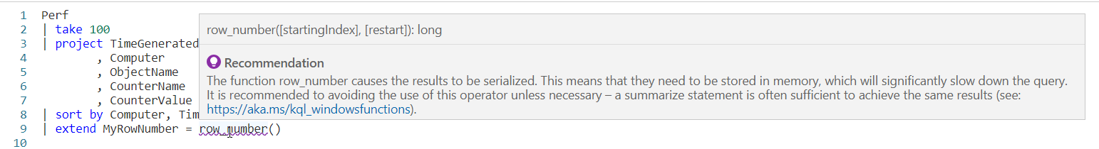
If you’ve not read my introductory post on Windowing Functions, Fun With KQL Windowing Functions – Serialize and Row_Number yet, you should do so now as it introduced several important concepts needed to understand how these Windowing Functions work.

The samples in this post will be run inside the LogAnalytics demo site found at https://aka.ms/LADemo. This demo site has been provided by Microsoft and can be used to learn the Kusto Query Language at no cost to you.

If you’ve not read my introductory post in this series, I’d advise you to do so now. It describes the user interface in detail. You’ll find it at https://arcanecode.com/2022/04/11/fun-with-kql-the-kusto-query-language/.

Note that my output may not look exactly like yours when you run the sample queries for several reasons. First, Microsoft only keeps a few days of demo data, which are constantly updated, so the dates and sample data won’t match the screen shots.

Second, I’ll be using the column tool (discussed in the introductory post) to limit the output to just the columns needed to demonstrate the query. Finally, Microsoft may make changes to both the user interface and the data structures between the time I write this and when you read it.

Row_Window_Session Basics

The row_window_session function allows you to group data into time based groups. It will find the beginning of a time group, which KQL calls a session, then will return the beginning time of the session (along with other data) until the conditions are met to cause a new session to start.

Let’s look at an example query, then we’ll break down the various parts.

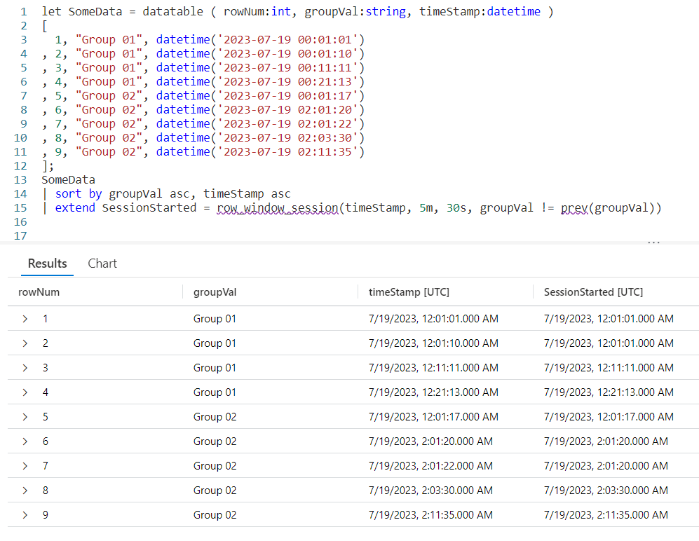
We begin by declaring a datatable to hold our sample data. It has three columns. The rowNum is included to make it easier to discuss the logic of row_window_session in a moment, otherwise it’s just an extra piece of data.

I then include a groupVal column. It will be used to trigger the beginning of a new time group (aka session). Working with real world data, you may use something like the name of a computer for the group.

Finally we have a column of datatype datetime. When working with log data from, for example, the Perf table this would typically be the TimeGenerated column but it doesn’t have to be. Any datetime datatype column can be used. I’ve crafted the data to make it easier to explain how row_window_session works.

Next, I take our SomeData dataset and pipe it into a sort, sorting by the group and time in ascending order. The sort has the added benefit of creating a dataset that is serializable. See my previous post on serialization, mentioned in the introduction, for more on why this is important.

Finally we fall into an extend where we create a new column I named SessionStarted. We then assign it the output of the row_session_started function, which requires four parameters.

The first parameter is the datetime column to be used for determining the session window. Here it is timeStamp. The next three parameters are all conditions which will trigger the beginning of a new “session” or grouping.

The second parameter is a timespan, here I used a value of 5m, or five minutes. If more than five minutes have elapsed since the current row and the first row in this group, it will trigger the creation of a new window session (group).

The third parameter is also a timespan, and indicates the maximum amount of time that can elapse between the current row and the previous row before a new window session is started. Here we used 30s, or thirty seconds. Even if the current row is still within a five minute window from the first row in the group, if the current row is more than thirty seconds in the future from the previous row a new session is created.

The final parameter is a way to trigger a change when the group changes. Here we use the groupVal column, but it’s more likely you’d use a computer name or performance counter here.

Breaking it Down

Since this can get a bit confusing, let’s step through the logic on a row by row basis. You can use the rowNum column for the row numbers.

Row 1 is the first row in our dataset, with a timeStamp of 12:01:01. Since it is first, KQL will use the same value in the SessionStarted column.

In row 2, we have a timeStamp of 12:01:10. Since this is less than five minutes from our first record, no new session is created.

Next, it compares the timeStamp from this row with the previous row, row 1. Less than 30 seconds have elapsed, so we are still in the same window session.

Finally it compares the groupVal with the one from row 1. Since the group is the same, no new session window is triggered and the SessionStarted time of 12:01:01, the time from row 1 is used.

Now let’s move to row 3. It has a time stamp of 12:11:11. This is more than five minutes since the time in row 1, which is the beginning of the session, so it then begins a new window session. It’s time of 12:11:11 is now used for the SessionStarted.

Row 4 comes next. It’s time of 12:21:13 also exceeds the five minute window since the start of the session created in row 3, so it begins a new session.

Now we move into row 5. Because the groupVal changed, we begin a new session with a new session start time of 12:01:17.

In row 6 we have a time of 02:01:20. Well a two am time is definitely more than five minutes from the row 5’s time, so a new session is started.

The time in row 7 is 02:01:22. That’s less than five minutes from row 6, and it’s also less than 30 seconds. Since it is in the same group, no new session occurs and it returns 02:01:20 for the SessionStarted.

Now we get to row 8. The time for this row is 02:03:30, so we are still in our five minute window that began in row 6. However, it is more than 30 seconds from row 7’s time of 02:01:22 so a new window session begins using row 8’s time of 02:03:30.

Finally we get to row 9. By now I’m sure you can figure out the logic. Its time of 02:11:35 is more than five minutes from the session start (begun in row 8), so it triggers a new session window.

Remember the Logic

While this seems a bit complex at times, if you just remember the logic it can be pretty easy to map out what you want.

Did the group change as defined in the fourth parameter? If yes, then start a new window session.

Compared to the session start row, is the time for the current row greater in the future by the value specified in parameter 2? Then start a new window session.

Compared to the previous row, is the time for the current row farther in the future then the amount of time in parameter 3? If so, start a new window session.

TimeSpans

In this example I used small values for the timespans, 5m and 30s. You can use any valid timespan though, including days and hours.

For a complete discussion on the concept of timespans, see my blog post Fun With KQL – Format_TimeSpan.

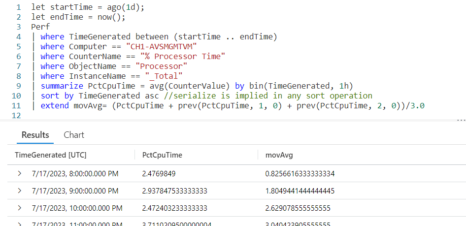
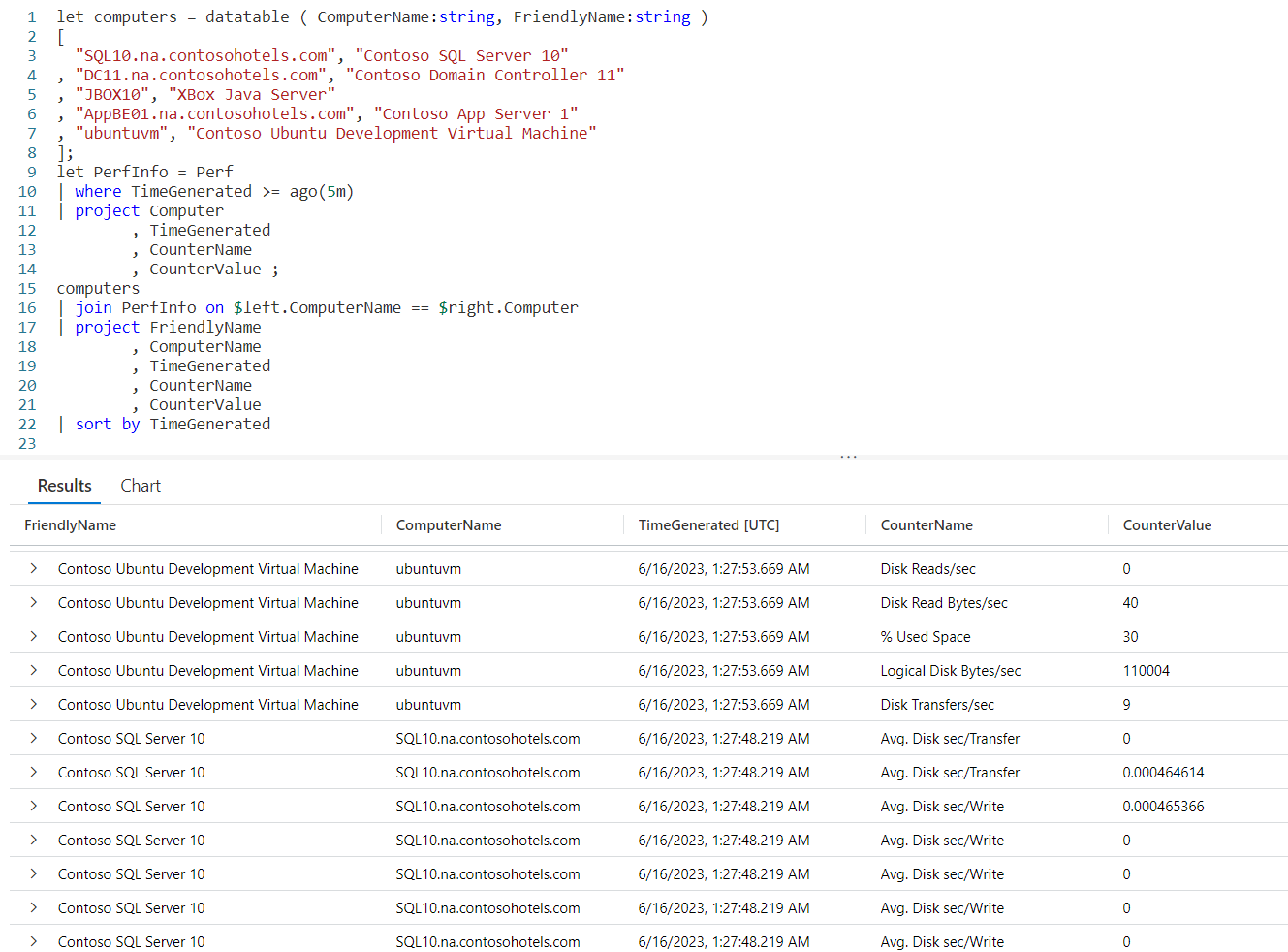
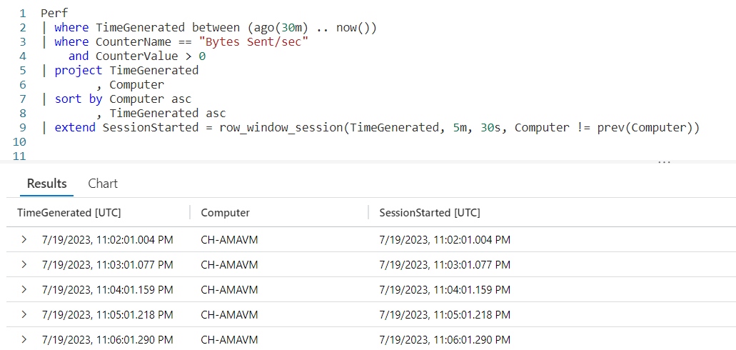
Let’s Use Real Data

For completeness I wanted to include a final example that uses the Perf table from the LogAnalytics demo website.

The logic is similar to the previous example. Since you now have an understanding of the way row_window_session works, I’ll leave it up to you to step through the data and identify the new window sessions.

Conclusion

With this post on row_window_session, we complete our coverage of Kusto’s Windowing Functions. You saw how to use it to group data into timespans based on a beginning date, with the ability to group on total elapsed time since the start of a window or since the previous row of data.

The demos in this series of blog posts were inspired by my Pluralsight courses on the Kusto Query Language, part of their Kusto Learning Path.

There are three courses in this series so far:

I have two previous Kusto courses on Pluralsight as well. They are older courses but still valid.

These are a few of the many courses I have on Pluralsight. All of my courses are linked on my About Me page.

If you don’t have a Pluralsight subscription, just go to my list of courses on Pluralsight. On the page is a Try For Free button you can use to get a free 10 day subscription to Pluralsight, with which you can watch my courses, or any other course on the site.

Fun With KQL Windowing Functions – Row_Rank_Dense

Introduction

The Kusto Windowing Function row_rank_dense is an interesting function. It lets you get a unique count of a specific column in a dataset. Unlike other methods of getting counts, row_rank_dense allows you to see each individual row of data.

First though, if you’ve not read the introductory post on Windowing Functions, Fun With KQL Windowing Functions – Serialize and Row_Number, you should do so now as it introduced several important concepts needed to understand how these Windowing Functions work.

Row_Rank_Dense Basics

The row_rank_dense is used to determine the density of a value. By passing in a sorted dataset, you can get a rank number for each item. The rank number changes only when the value we’re evaluating changes.

An example will make this much clearer. We start by creating a datatable with three columns. The rowNum is just used to make it easier to discuss the output in a moment. Likewise rowVal provides some easy to consume text.

The important column is valToRankOn. It is this value that is going to be evaluated within our row_rank_dense Windowing Function.

The SomeData dataset is piped into a sort, where we sort on the value we are evaluating in ascending order. We will also sort on the rowVal, so when we have two identical values in valToRankOn, we can display the output in a logical fashion. In a real world situation, this might be the name of computer or perhaps a counter of some kind.

Using a sort will also mark the data as serializable, which is required in order to use row_rank_dense. For more on serialization, see the Fun With KQL Windowing Functions – Serialize and Row_Number post I mentioned in the introduction.

Finally we fall into an extend, creating a new column Rank. We’ll assign it the output of our row_rank_dense function. In it we use one parameter, the name of the column to be evaluated, here it is valToRankOn.

In the output, our first row is row 7, with a valToRankOn of 1. Thus it is assigned a Rank of 1.

The next row is row 8, it has the next smallest value of 6 in the valToRankOn column, so it gets a Rank of 2.

Rows 6 and 9 both have the same valToRankOn, 17. Since 17 is the third smallest value, both rows are given a Rank of 3. Because we included rowVal in the sort, they are listed in order of the rowVal, Value 06 then Value 09.

This continues for the remaining rows of data. We can see both how many unique values we have, six, and still see each individual row of data.

Density by Largest Value

In the above example, by sorting the valToRankOn in ascending order the smallest values come first, then increase with a Rank of 1 being given to the smallest value.

If we had instead sorted valToRankOn in descending order, sort by valToRankOn desc, ..., then the Rank of 1 would have been assigned to the largest value, then as the valToRankOn decreased the Rank would have increased. I’ll leave it as an exercise for you to play with this by altering the sort order for your sample queries.

Grouping In Row_Rank_Dense

It is also possible to organize rankings within a group. For example, within a single computer you might want to rank a counter value. With the next computer you’d want the rankings to begin again. This would allow you to have rankings that are unique to each computer.

In the example below I’ve added a new column to the datatable named groupVal. We’ll be using this column for our grouping. It was also added to the sort operator so we’ll sort by group first, then the value to rank on, and finally the rowVal text.

The row_rank_dense function supports a second parameter, a boolean value that when true will trigger a new group to begin. Here we are using an equation, which will compare the groupVal for the current row to the one of the previous row using the prev Windowing Function. If they are not equal, the comparison will return true and trigger row_rank_dense to begin a new dense rank grouping.

In the output, rows 1 and 3 (from the rowNum column) have the same valToRankOn, so are both given the Rank of 1. The third row in this group, row 2, is assigned a Rank of 2.

With row 4, we see the groupVal has changed. So the row_rank_dense function reset and began a new ranking, assigning this row a Rank of 1.

When the group changes again in row 7, the Rank value is again reset to 1 and we work our way up.

Row_Rank_Dense in the Real World

Let’s take a look now at an example of using row_rank_dense for a “real world” query. Here, we are going to query the Perf table to bring back rows for the last five minutes where the CounterValue is Bytes Sent/sec, and we’ll remove any rows with a value of zero.

We’ll project each column we need and sort the data. Here we’ll again sort in ascending order so the smallest counter values come first, but we could just have easily sorted the CounterValue in descending order so the largest values came first.

When we call row_rank_dense, we’ll pass in the value we want to rank in the first parameter, CounterValue. In the second parameter we’ll compare the name of the computer in this row to the one of the previous row using the prev function. When they don’t match the comparison will return true, which will trigger the row_rank_dense function to begin a new group.

As you can see, we begin with computer CH-AMAVM, with its value of 2.26333 given the rank of 1, then the rank values increase as the counter values increase.

When we hit computer CH1-AVSMGMTVM, note the Rank reset itself. The first row for this computer, with a counter value of 2.34613 has a Rank of 1.

This pattern will repeat for the remaining rows of data from our query.

Conclusion

In this post you saw how to use the row_rank_dense Windowing Function to order and rank values in a dataset from smallest to largest, or largest to smallest.

The next and final post in the Kusto Window Functions series will cover the use of row_window_session to group and organize data into time windows.

The demos in this series of blog posts were inspired by my Pluralsight courses on the Kusto Query Language, part of their Kusto Learning Path.

There are three courses in this series so far:

I have two previous Kusto courses on Pluralsight as well. They are older courses but still valid.

These are a few of the many courses I have on Pluralsight. All of my courses are linked on my About Me page.

Fun With KQL Windowing Functions – Row_Rank_Min

Introduction

In this post we’ll cover the next in our series on KQL Windowing Functions, row_rank_min. The row_rank_min function will assign rank numbers to an incoming dataset, with the rank of 1 being assigned to the minimal value in the dataset and increasing as the values increase.

Row_Rank_Min Basics

We being by using let to define a datatable with some values to use for our example. The rowNum and rowVal are just included to have some data to look at.

The important column is valToRankOn. This is the column that will be evaluated and used to rank the data. Let’s see how our query works.

We take our SomeData and pipe it into a sort, sorting by the value to rank on and the row value (rowVal). Note we need to sort the valToRankOn in ascending order to get the row_rank_min to work correctly, and while we are at it we’ll sort the rowVal in ascending order as well.

The sort has the added benefit as making the data serializable, so it can be used with KQL Windowing Functions, in this case row_rank_min. For more on serialization see the post I referenced in the introduction, Fun With KQL Windowing Functions – Serialize and Row_Number.

After the sort we have an extend where we create a new column Rank. To it we assign the output of row_rank_min. Into the function we pass the column to evaluate for the rank, here we are using valToRankOn.

The smallest value is given a rank of 1, as you can see with rowNum 7. The next smallest value, found on rowNum 8 is assigned a rank of 2. Row 3 has a valToRankOn of 15, which is the next smallest value so it was given a rank of 3.

Rows 6 and 9 both have a value of 17, so both are assigned the same minimal rank number of 4. Because we added the rowVal to the sort, the rows are sorted in ascending order by the rowVal within the Rank of 4.

This pattern is repeated for the remaining rows, with the rank value increasing as the values in valToRankOn increases. As you can see, this provides an easy way to rank values from smallest to largest.

Ranking Within a Group

Similar to the row_cumsum Windowing Function we looked at in the previous post, we can create rankings within a group. In the following sample, a new column of groupVal was added to the SomeData sample dataset.

In the example we made two changes from the previous sample. First, the groupVal was added to the sort statement.

The next change occurred in the row_rank_min function. It supports a second parameter that will trigger a reset of the ranking value. It needs to evaluate to a boolean true/false value. When true, it resets the ranking value.

Here, we are comparing the groupVal of the current row to the groupVal of the previous row using the prev function. If the group name for the current row is different from the previous row, the comparison will return true since they are not equal. This will trigger the ranking to restart.

In rowNum 4 the group changes to Group 2, so Kusto starts the ranking again. Within Group 2, the value of 22 on row 4 is the smallest, so it gets the rank of 1.

This technique lets us create minimal ranking values within individual groups of data. Here we are using groupVal, in a real world you might use something like a computer name or performance counter name.

Real World Example

In this query we’ll create something you might use in the “real world”. We’re going to look at the Perf table for the counter “Bytes Sent/rec”, where there is data (the counter value is greater than zero).

We’ll project only the columns we need, then sort the output. We want to create rankings for each computer, from the smallest counter value to the biggest. By doing so we can easily see what times we had the smallest and largest values.

Here we use row_rank_min to evaluate the CounterValue. In the second parameter we are checking to see if the Computer name has changed, if so the rank will reset for the next computer.

Looking at one example, when the Computer changed from CH-AMAVM changes to CH1-AVSMGMTVM, the rank reset so the smallest value of 16.4175 is given the rank of 1.

Conclusion

With this post we saw how to create rankings for values using the row_rank_min function. This allows us to easily identify the smallest value, with a rank of 1 and work up to the largest value.

In our next post we’ll continue our KQL Windowing Function series by looking at the row_rank_dense function, which is similar to this posts row_rank_min.

The demos in this series of blog posts were inspired by my Pluralsight courses on the Kusto Query Language, part of their Kusto Learning Path.

There are three courses in this series so far:

I have two previous Kusto courses on Pluralsight as well. They are older courses but still valid.

These are a few of the many courses I have on Pluralsight. All of my courses are linked on my About Me page.

Fun With KQL Windowing Functions – Row_CumSum

Introduction

Seeing cumulative totals on a row by row basis is a common need. Think of your bank account, when you look at your ledger it shows each individual transaction. Beside each individual transaction is the current amount in your account, as offset by the amount of the current transaction.

This technique is known as cumulative sums. The Kusto Query Language provides the ability to create cumulative sums using the Windowing Function, row_cumsum. In this post we’ll see how to implement it.

If you’ve not read my introductory post in this KQL series, I’d advise you to do so now. It describes the user interface in detail. You’ll find it at https://arcanecode.com/2022/04/11/fun-with-kql-the-kusto-query-language/.

Row_CumSum Basics

For this example I’ll be using let to generate a simple dataset using the datatable operator. It will have two columns, the row number rowNum, and a value rowVal. For more information on let, datatable, serialize, and other functions used in this post refer to the See Also later in this post.

Using row_cumsum is simple. First, we need to pipe the dataset SomeData into a serialize so we can use it with Windowing Functions. The serialize also lets us create a new column we named cumSum, and set it equal to the row_cumsum output. As a parameter, I pass in the numeric column I want to add up, here I used the rowNum column.

As you can see in row 1, the row number (rowNum) has a value of 1. There is no data since there are no previous rows, so it just returns 1.

In the second row, the value of rowNum is 2. The cumSum column already had a value of 1, so we’ll add 2 to it, for a result of 3.

With the third row, we’ll add the value in rowNum (3) to the value in cumSum (which also happened to be 3) and we’ll now have a cumulative sum of 6.

This repeats for each row, creating a cumulative summary.

You can also create a way to decrement the data by using a negative value for the row_cumsum parameter. For example, row_cumsum(rowNum * -1) could have been used to create a decrementing value much as spending money out of your checking account would decrement your balance. You’d just want to determine the best way to handle the beginning value (first row) of the dataset.

Resetting the Cumulative Counter

It’s possible you may not want to keep accumulating for all rows, but instead only have the accumulation for a group of rows. A common task is to reset the sum when a computer name changes, or perhaps the calendar month.

For this example, I’ve added a third column to our datatable, rowBucket. Whenever the value in rowBucket changes, I want to reset the cumulative sum value.

The row_cumsum supports a second parameter that is a boolean value. When true, the counter resets. Here, I’m using an equation to calculate “is the current rows rowBucket value not equal to the one from the previous row”. If this is true, in other words not equal, then the counter will reset.

Sure enough, on row 4 the rowBucket changed to 2. On this row the cumulative sum reset itself. It now keeps adding up until the bucket number changes again, as it does with row 6.

A Real World Example

Using a datatable made the examples easy to understand, but it’s time to look at an example you might want to use in the “real world”.

Let’s imagine a scenario where you’ve detected a large amount of network traffic coming from one of the computers on your Azure network. You’d like to check the performance log table (Perf) to see how many bytes each computer sent in the last five minutes.

You need to see the number of bytes sent by a computer for each log entry, but you also want to see the total bytes sent by a computer for that time period. Let’s look at a query to accomplish this goal.

We begin with our old buddy the Perf table. A where will limit the data to the last five minutes. A second where will limit the counter to just the one we are interested in, Bytes Sent/sec. Since we only need to see this data when the virtual Azure server sent data, we’ll add a final where to remove any rows where the CounterValue is zero.

Next, we’ll use a project to strip down the columns to only the three we are interested in: the Computer, TimeGenerated, and CounterValue.

We then want to use a sort, so the data for each computer will be grouped together, then within a Computer the time the performance data was generated. Note that since the default for a sort is descending order, an asc was added after the TimeGenerated so the entries would go from the oldest to the most recent.

I normally might include an asc after the Computer so the computer names would be sorted alphabetically from A to Z, but left it off for this example just to remind you that with a sort you can mix and match the asc and desc columns.

Using a sort has another benefit. If you did go back and read my post Fun With KQL Windowing Functions – Serialize and Row_Number as I suggested in the introduction, you’ll know that the sort marks a dataset as safe for serialzation. In order to use Windowing Functions, such as row_cumsum and prev, a dataset needs to be safe for serialization.

The final line of the query is where the magic happens. Since using sort eliminated the need to use serialize, we can just use an extend to create a new column. I chose to name it cumulativeBytes.

We assign it the output of our row_cumsum Windowing Function. In the first parameter we pass in the CounterValue. In the second column we create an expression that will evaluate to true or false. We compare the Computer column for the current row and call the prev Windowing Function to get the Computer from the previous row of data.

If they are not equal, then the equation returns true. This will cause the row_cumsum to reset the cumulative sum.

Looking at the output, you can indeed see that occurred. The first computer in the list is CH1-VM-CTS. With each row it begins accumulating the CounterValue into the cumulativeBytes column.

When the Computer changed to CH-DMAVM, you can see the cumulativeBytes counter was reset. It kept accumulating the values for CH-DMAVM until the Computer changed to CH-AVSMGMTVM at which point it was again reset, and the pattern continues.

Conclusion

Cumulative sums are not an uncommon need when retrieving data. Kusto provides this ability with the Windowing Function row_cumsum, which you saw how to use in this post.

Our next post will continue the coverage of Kusto Windowing Functions by looking at the row_rank_min function.

The demos in this series of blog posts were inspired by my Pluralsight courses on the Kusto Query Language, part of their Kusto Learning Path.

There are three courses in this series so far:

I have two previous Kusto courses on Pluralsight as well. They are older courses but still valid.

These are a few of the many courses I have on Pluralsight. All of my courses are linked on my About Me page.

Fun With KQL Windowing Functions – Prev and Next

Introduction

In this post we’ll continue our series on Kusto’s Windowing Functions by covering prev and next. If you’ve not read the introductory post, Fun With KQL Windowing Functions – Serialize and Row_Number, you should do so now as it introduced several important concepts needed to understand how these functions are used.

So what do prev and next do? They allow you to retrieve a value in a column from a previous row, or the next (or upcoming) row. This can be very useful in many situations. For instance, calculating the time between two rows based on a datetime column, or the change in a value from one row to the next.

Prev Basics

To make these examples simple, I’m going to use the datatable operator to generate a very simple dataset. For more on how datatable works, please see my post Fun With KQL – Datatable.

Using a let, I’ve created a dataset named SomeData. It has nine rows and two columns: rowNum and rowVal.

After my let, I take the SomeData dataset and pipe it into a serialize so it can be used with Windowing Functions like prev. Refer back to my previous post on serialize for more information on how serializing a dataset lets you use Windowing Functions.

Now the data pipes into an extend, where we add a new column I named prvVal (short for previous value). We then use strcat to combine a text string, Previous Value was with the output of our prev Windowing Function.

Into prev we pass one parameter, the name of the column from the previous row we want the data for. Here we want to pull data from the column rowVal.

As you can see in the output, the right most column displays our Previous Value was text string, plus the value from the rowVal column in the previous row.

Even More Previous

We can go back more than just one row. The prev function supports a second parameter that indicates the number of rows to go back.

First, I decided to use two extends. The first will copy the previous value into a variable, prvVal2. Into the prev function I pass two values, the first is the column name we want the data from. Here we’ll use rowVal again. The second parameter is the number of rows we want to go back, in this case we just used the value of 2.

In the next extend I user strcat to combine the prvVal2 variable with a text string and put it into the new column prvValOutput. I did this just to demonstrate you could pull a value from a previous row and use it in the query. I could have done other things with prvVal2, such as use it in a calculation.

Previous Value? What Previous Value?

You probably noticed that when we are on the first row, there is no previous value. Likewise, when on the first or second rows, and going back two there was no data. In this case the prev just returned a null value.

In the past I’ve written about functions like iif and isnull to help handle null values. Fortunately, prev eliminates the need for these as it supports and optional third parameter. Into it you can supply a value to use when the value returned by prev would otherwise be null.

In our prev we first pass the column from the previous row we want the data from, rowVal. In this example we are only going to go back one row, but since we want to use the third parameter we have to supply a value in the second parameter position. In this example we’ll use the number 1.

Finally in our third parameter we supply a value to be returned when the result of a prev would be null. Here we used the text not valid for this row, although we could have used a different datatype such as a numeric value or a datetime if that would have been more appropriate to our query.

Next, let’s look at next. The next function behaves just like prev, except it will get data from the next row in our serialized dataset instead of a previous row.

Just like with prev, as the parameter to next we pass in the name of the column to get the data from.

The next function also supports the optional second and third parameters. The second being a number indicating how many rows to go forward, the third being a value to use when next would otherwise return a null value.

Since you’ve already seen these in play I won’t create samples here, but you should be able to easily create them for yourself following the examples from prev.

Calculating a Moving Average

So it’s time for a more realistic example. Here I want to get the % Processor Time from the Perf table for a particular computer. I’m going to summarize it by hour. Then I want to create a moving average for the last three hours.

Most of the query will be pretty straightforward if you’ve been following my KQL series. I capture a start and end time using let. I then use the Perf table, followed by several where statements to limit the data.

Next I use summarize to create an average, bucketed by hour. In essence I’ll have an average of all the processor times for the 1 am hour, then 2 am, and so on.

After that we’ll sort them by the time of the day. Not only will the sort put the data in the order we want, it will also mark them as serialized. This means we can use them with our Window Function prev.

The last line is where the exciting things happen, so take a look and we’ll break it down.

We begin with extend in order to create a new column, movAvg. We are then going to add three values. The first value is the PctCpuTime from the current row, which was calculated during the summarize.

Next, I want to add in the PctCpuTime from the previous row. To do that we’ll use the prev function, pass in the PctCpuTime as the column to get, 1 to indicate we want to go back one row, then tell it to return a 0 (zero) when the previous row would return null.

This is then repeated only we pass in a value of 2, indicating we should go back two rows.

After the closing parentheses we divide by 3.0. Note its important to include the .0 otherwise it would try to create an integer output and we want a full decimal value.

And there you go, we now have an average for the last three rows of data.

Let me acknowledge, by returning a 0 for missing (null) values from the prev, the averages for the first two rows will be off. In a real world situation you’d want to make sure to take this into account, creating a solution appropriate to your situation. For this example I used zero in order to keep things simple.

Conclusion

This post continued our journey with KQL Windowing Functions, seeing how the useful prev and next functions could get data from adjacent rows of a serialized dataset. In our next post we’ll be looking at a Windowing Function to let us get cumulative sums.

The demos in this series of blog posts were inspired by my Pluralsight courses on the Kusto Query Language, part of their Kusto Learning Path.

There are three courses in this series so far:

I have two previous Kusto courses on Pluralsight as well. They are older courses but still valid.

These are a few of the many courses I have on Pluralsight. All of my courses are linked on my About Me page.

Fun With KQL Windowing Functions – Serialize and Row_Number

Introduction

The Kusto Query Language includes a set of functions collectively known as Window Functions. These special functions allow you to take a row and put it in context of the entire dataset. For example, creating row numbers, getting a value from the previous row, or maybe the next row.

In order for Window Functions to work, the dataset must be serialized. In this post we’ll cover what serialization is and how to create serialized datasets. This is a foundational post, as we’ll be referring back to it in future posts that will cover some of the KQL Windowing Functions.

Serialization

When a dataset is serialized, its data is placed in a specific order and that order is retained as the dataset goes through various transformations. Some of the Windowing Functions that require a serialized dataset to work are row_number, next, and prev to name just a few that will be covered in this and future posts.

There are some KQL functions that by their nature emit a dataset that is already ordered, in other words serialized. These include functions that I’ve already written about such as top and sort.

There are also some operators that if they receive a serialized dataset as input, will preserve the serialized ordering when the data is output. I’ve written about all of these in past posts, and they include: extend, mv-expand, parse, project, project-away, project-rename, take and where.

So the big question is, what if I need to use a Window Function but my data is not already serialized?

The Serialize Operator

For situations when you do not have an already serialized dataset you can easily create one using the serialize operator. Here’s a simple example.

All we have to do is take our dataset and pipe it into the serialize operator. The dataset will then have its order preserved, and will mark the dataset safe for use with KQLs Windowing Functions, similar to when a social media site lets you mark yourself safe from a hurricane, tornado, or all night HeavyDSparks marathon on YouTube. (#GuiltyPleasures)

Of course we don’t see any visible change here, but now we can use it with a Windowing Function. If you peeked at the post title, you’ve probably guessed already that for this post we’ll use the Window Function row_number.

But first…

A Warning!

Eagle eyed readers may notice the serialze in the screen shot above is underlined with red squiggles. This indicates there is a warning associated with this operator.

If we hover over the serialize operator the interface will display the specific warning to us.

It’s letting us know that in addition to being marked safe for Kusto Window Functions, the dataset will also be stored in memory. This could adversely affect the query runtime.

Sometimes it’s necessary to use serialize in order to get the results you need, but keep it in mind. Should you have a slow running query think about reducing the size of the dataset or see if there are other ways to accomplish the same results.

That said, let’s see how to use a basic Window Function, the row_number.

Row_Number

Calling the row_number function is easy. After the serialize operator we first provide a new column name that will hold our row number, here I used MyRowNumber. I then assign it the function row_number(). Note because it is a function we have to include the parenthesis after the function name.

In the very right most column you can see our new row number column, MyRowNumber. The value is incremented with each row.

Row_Number Without Serialize

It’s possible to call the row_number function without using the serialize operator. As discussed earlier in this post the Windowing Functions need a serialized dataset to work with, and there are a few operators that will produce a dataset that is already safe to be serialized, such as top and sort.

In addition we have the operators that will preserve serialization when a serialized dataset is passed in. As a refresher these operators include: extend, mv-expand, parse, project, project-away, project-rename, take and where.

In this example, we’ll use a sort to get our data in the order we want, then use an extend to add the new MyRowNumber column by calling the row_number() function.

As you can see, after the sort we call extend and use the same syntax as before, creating the new column of MyRowNumber and assigning it the function row_number(). Looking to the right you can see the new MyRowNumber column in the output.

You also may notice the row_number function now has a red squiggly line under it, indicating a warming. Let’s go see what that’s all about…

Another Warning!

Hovering over the row_number displays the following warning:

This warning is similar to the one you saw when we used the serialzie operator. It states that by calling row_number the data will be stored in memory, which could slow down the query.

It does have an interesting implication though. Using sort means the data can be serialized, but doesn’t mean it is. The warning states it’s the calling of a Windowing Function, such as our new friend row_number, that actually triggers the data to be serialized.

Serialize and Window Functions Recap

When we talk about Windowing Functions, I wanted to stress an important point. The serialize operator is used to convert a dataset that is not already safe for serialization into one that is. The serialization is required in order to use a Windowing Function such as row_number or one of the other’s we’ll cover in this series.

There are a list of other operators though that output data that is already safe for serialization, in other words if we use one of these operators then we can use a Windowing Function without the need to use serialize. I mentioned top and sort already, but for completeness here is the full list.

top
sort
range
getschema
top-hitters

I’ve already done blog posts for the first two (you can click on the command to follow the link to the post), and have one planned for range. If there’s interest I may cover the other two.

For completeness, let me go ahead and list the operators that will preserve the serialized state of the data when used. Note each is linked to a blog post I’ve done previously which covers each operator.

Conclusion

In this post we learned hot to use serialize to create a dataset with which we can call one of the Kusto Languages Windowing Functions. We also learned there are a handful of operators that already produce datasets safe for serialization, and can be used with Windowing Functions without the requirement to use the serialize operator.

Finally we saw the row_number Windowing Function in action. In future posts we’ll cover more of the Windowing Functions built into the Kusto Query Language.

The demos in this series of blog posts were inspired by my Pluralsight courses on the Kusto Query Language, part of their Kusto Learning Path.

There are three courses in this series so far:

I have two previous Kusto courses on Pluralsight as well. They are older courses but still valid.

These are a few of the many courses I have on Pluralsight. All of my courses are linked on my About Me page.

Fun With KQL – Datatable and Calculations

Introduction

In the conclusion of my last post, Fun With KQL – Datatable, I mentioned a datatable can also be useful when you need to do special calculations. I decided it really needed further explanation and created this post to dive in a bit deeper.

If you haven’t read my datatable post yet, you should as I’ll refer back to it. Go ahead, I’ll wait.

Datatable and Calculations

For this example we’ll revisit the Perf table. The Perf table has two main columns that we’ll use in this example, CounterName and CounterValue.

Our goal for this query is to multiply the CounterValue by some number, based on the CounterName. We could of course use a case or iif within the query, but that would result in a query that is long and hard to read and later modify if we need to.

Using a datatable will result in a query that is much more readable and maintainable. As the actual code for the query is a bit long I’ll place it below to make it easy to follow along. Note I’ll only skim over things we covered in the previous post, refer to it for more detailed explanations.

let CounterMultipliers = datatable (CounterName:string, Multiplier:int)
[
  "CounterName", 2,
  "restartTimeEpoch", 3,
  "memoryWorkingSetBytes", 4,
  "memoryRssBytes", 5,
  "memoryRequestBytes", 2,
  "memoryLimitBytes", 3,
  "memoryCapacityBytes", 4,
  "memoryAllocatableBytes", 5,
  "cpuUsageNanoCores", 2,
  "cpuRequestNanoCores", 3,
  "cpuLimitNanoCores", 4,
  "cpuCapacityNanoCores", 5,
  "cpuAllocatableNanoCores", 2,
  "Total Bytes Transmitted", 3,
  "Total Bytes Received", 4,
  "Logical Disk Bytes/sec", 5,
  "Free Megabytes", 2,
  "Disk Writes/sec", 3,
  "Disk Write Bytes/sec", 4,
  "Disk Transfers/sec", 5,
  "Disk Reads/sec", 2,
  "Disk Read Bytes/sec", 3,
  "Disk Bytes/sec", 4,
  "Bytes Sent/sec", 5,
  "Bytes Received/sec", 2,
  "Avg. Disk sec/Write", 3,
  "Avg. Disk sec/Transfer", 4,
  "Avg. Disk sec/Read", 5,
  "Available MBytes Memory", 2,
  "Available MBytes", 3,
  "% Used Space", 4,
  "% Processor Time", 5,
  "% Free Space", 6
];
let PerfData = view() {
Perf
| project CounterName
        , CounterValue
        , Computer
        , ObjectName
        , TimeGenerated
};
PerfData
| join CounterMultipliers on CounterName
| project CounterName
        , CounterValue
        , Multiplier
        , CounterExpanded = CounterValue * Multiplier
        , Computer
        , ObjectName
        , TimeGenerated

We begin with a let, where we will create a new datatable. I chose to name it CounterMultipliers, but we could have used any name we wanted.

The datatable will have two columns, the CounterName which is a string, and the Multiplier which I made an int.

I used a simple query to get the list of CounterName values:

Perf
| distinct CounterName
| sort by CounterName

I then copied the output into my query editor. I wrapped the names in quotes so they would be interpreted as strings. Next I have a comma, then the integer value to use for the multiplier.

Note I just picked a few random values to use here. In a real world situation this kind of operation, multiplying counter values, might not make much sense, but it will serve OK for this example.

After finishing the datatable definition I use a second let to create a temporary view on top of the Perf table and named the view PerfData. For more on this technique refer back to the Fun With KQL – Datatable post.

Now we take our PerfData view and join it to our datatable, CounterMultipliers. Note that I used the best practice of naming the counter name column in the datatable the same as in the PerfData view. It makes the query easier to read, and avoids the need for $left and $right as I described in the previous post.

Finally we pipe the output of the join into a project operator. I return all the columns, but add a new one, CounterExpanded. For its calculation I simply take the CounterValue column from the PerfData view and multiply it by the Multiplier column from the `datatable.

Below you can see the output from the query.

If you look in the lower right though, you will spot an issue. The query only returned 32 rows.

This demonstrates a critical piece of information when it comes to the join. For each row in the first table, PerfData, it grabs a row from the second table. Since we had 32 rows in the datatable, only 32 rows were returned.

Fixing the Query

Fixing the query is simple. All we need to do is swap the order of the two tables.

CounterMultipliers
| join PerfData on CounterName
| project CounterName
        , CounterValue
        , Multiplier
        , CounterExpanded = CounterValue * Multiplier
        , Computer
        , ObjectName
        , TimeGenerated

Note I only included the last part of the query, everything above this piece is still the same.

Now look at the output.

In the lower right, as well as in the blue area at the top of the output, you can see over 300,000 rows were returned. This is the output we expect, every row in the Perf table (from the view) linked to each row in the CounterMultipliers datatable.

Including and Excluding Columns

In this example, in the output I included the Multiplier column. This was done so you could see the data and test the calculation for yourself. In a normal situation you likely wouldn’t be doing this.

I also included the CounterValue column. Again, this may or may not be needed, you could choose to have just the CounterExpanded column.

Think about the output, and how it will be used to decide if you want to include these types of columns in your query output.

Conclusion

In this post we learned how to use a datatable to create calculated values. This made the code much cleaner, and easier to read.

The demos in this series of blog posts were inspired by my Pluralsight courses on the Kusto Query Language, part of their Kusto Learning Path.

There are three courses in this series so far:

I have two previous Kusto courses on Pluralsight as well. They are older courses but still valid.

These are a few of the many courses I have on Pluralsight. All of my courses are linked on my About Me page.

Fun With KQL – Datatable

Introduction

As you’ve seen with the join in my Fun With KQL – Join post it can be useful to combine two tables in order to clarify the output. What if, though, you need data that isn’t in an existing table?

That’s where the datatable operator comes into use. The datatable allows you to create a table of data right within the query. We’ll see a few useful examples in this post.

DataTable Basics

Let’s say you have a table that stores colors. These colors though are stored in decimal format, the application that uses them converts them to an HTML hex color. For our report though, we’d like to convert these to a friendly name, which is not stored in the source data.

To accomplish this we can create a color table with the codes as well as friendly color names. We’ll use the datatable operator to do this.

We’ll need to use our old friend let. Following we declare a name for our datatable, here we used HTMLColors although we could use any name we want.

After the equal sign we use the datatable operator. In the parenthesis we declare our column names and their data types. The first is Name, then a colon, then the data type of string. Our second column is also a string, with the name of HexCode.

The final column is DecimalValue, and its datatype is int. You can find a complete list of Kusto data types in the Microsoft documentation, Scalar data types.

After we finish the datatable declaration with a closing right parenthesis, we have an opening square bracket then declare our data. Here I put each row of data on a line by itself, this is a good practice to make it easy to read and modify.

As you can see, our first row is:

"Red",	"#FF0000", 16711680,

First is what I call our friendly name associated with the color, followed by a comma. We wrapped it in double quotes, since it is a string datatype.

Then we have the hex color code, also wrapped in quotes to make it a string, followed by a comma. Finally comes the decimal value, which is just an integer number, no quotes required.

Then line ends in a comma, then we proceed to the next line of data. At the end of our data, the row with Aquamarine, we do not have a comma since that is the last row of data. We have a closing square bracket to finish off the datatable data, then a semicolon as the KQL query will continue.

Next have the name of our datatable, piped into a project, then we listed the three columns in the datatable.

As you can see in the image above, the output section has a list of colors, hex values, and decimal value. Note that a few scrolled off the bottom of the screen.

Now we could join this to a table, linking on the DecimalValue column and display the friendly Name column in the output.

Datatable In Practice

Let’s look at an example of the datatable in practice. The Perf table has a column, ComputerName. A lot of the computer names are rather cryptic though. It’d be nice to have a friendly, human readable name that clearly says what the computer is used for, rather than unclear like JBOX10.

Let’s take a look at the query needed to add friendly names to our Perf table output.

We begin with a let and define a datatable we’ll call computers. It will have two columns, ComputerName and FriendlyName, both of which are strings.

We fall into our data, each line is simply the computer name as found in the Perf table, followed by the friendly name we want to use.

Next comes another let in which we create a datatable from Perf for the last five minutes, and use project to pick out a few columns. We’ve named this datatable PerfInfo.

Now we take our computer datatable and join it to PerfInfo. Because the column we are joining on has different names in each table, I had to use the $left and $right, as described in my Fun With KQL – Join post.

We then project the columns we want, and use sort to order the output.

I should mention I just guessed at the friendly names for some of the computer names in the Perf table. I have no idea if JBOX10 is really the XBox Java Server, but it just sounded good for this demo.

Naming DataTable Columns

I just wanted to mention that normally I would use the same column name in the datatable that is used in the table I’m joining. For example, I would use just Computer in the datatable so it would match up with the Computer column in the Perf table. That way I wouldn’t have to use the $left and $right syntax.

For this example though, I deliberately used a different name so I could remind you of the ability to use $left and $right to join tables when the column name is different.

The most frequent time you’d need this is when you are joining multiple tables with different column names for the same data, which as anyone who has worked with databases for any length of time happens far too often.

Again, for more information on this technique see my Fun With KQL – Join post.

Conclusion

The datatable can be a useful operator for situations where you want to provide user friendly names, but don’t have an existing table that contains them.

It could also be used if you needed to do calculations. For example, rather than using iif statements you could create a datatable with a country code and a standard shipping amount, then in the table use that shipping amount in a calculation, perhaps adding it to the total value of a purchase.

The demos in this series of blog posts were inspired by my Pluralsight courses Kusto Query Language (KQL) from Scratch and Introduction to the Azure Data Migration Service, two of the many courses I have on Pluralsight. All of my courses are linked on my About Me page.

If you don’t have a Pluralsight subscription, just go to my list of courses on Pluralsight . At the top is a Try For Free button you can use to get a free 10 day subscription to Pluralsight, with which you can watch my courses, or any other course on the site.

Fun With KQL – Union Modifiers

Introduction

In my previous post, Fun With KQL – Union I covered how to use the union operator to merge two tables or datasets together. The union has a few helpful modifiers, which I’ll cover in this post.

The Kind Modifier

By default, when executing a Kusto Query if a column is null for every row in the result, that column is not displayed in the output. This is the behavior when using union without the kind a modifier. By default the kind modifier is set to kind=inner.

It is possible to force the union to display all columns, even if all the values for a column are null. To do so, after the union add kind=outer as shown in the example below.

Unfortunately, there’s not enough space to display all the output, but if you execute your own queries you’ll find columns for which every value is null in the output.

As a side note, the order of the modifiers isn’t important. The withsource could have been placed before the kind, for example.

The IsFuzzy Modifier

We’ve all been there. You have a query that’s been working fine, then all of a sudden it fails because someone deleted a table.

You may also be in a situation where you wish to union two tables, but the second table is a temporary table. Sometimes its there, sometimes not. You’d like to write a query to handle it.

Fortunately union has a modifier, isfuzzy. When you set it to true, it will successfully execute the query even if the second table is absent.

In this example I will union two tables, Update and ArcaneCode. Obviously there is no table named ArcaneCode in the LogAnalytics sample database.

As you can see, Kusto still executed the query successfully. It simply ignored the absence of ArcaneCode.

Putting It All Together

I’ll wrap this series on union up with a more complex but real world example. This query might be one you want to use for troubleshooting. Let’s look at the query first, then we’ll see the results.

let compName = "JBOX10";
let dateDiffInDays = ( date1:datetime, date2:datetime = datetime(2023-01-01) )
                     { 
                       (date1 - date2) / 1d 
                     };
let UpdtSum = view() {
  UpdateSummary
  | where Computer == compName
  | project Computer
          , ComputerEnvironment
          , ManagementGroupName
          , OsVersion
          , Resource
          , ResourceGroup
          , SourceSystem
          , Type
          , NETRuntimeVersion
          , TimeGenerated
  } ;
let Updt = view() {
  Update
  | where Computer == compName
  | project Computer
          , ComputerEnvironment
          , ManagementGroupName
          , OSVersion
          , Resource
          , ResourceGroup
          , SourceSystem
          , Type
          , Title
          , UpdateState
          , TimeGenerated 
  } ;
union withsource = "SourceTable"
      UpdtSum
    , Updt
| extend DaysSinceStartOfYear=dateDiffInDays(TimeGenerated)

It begins with a let, in which we define a variable, compName, to hold the name of the computer we want to get data for. This will make it easy to reuse the query with other computers.

In the next let we will create our own function to calcuate the difference between two dates. I’ll cover functions in more detail in a future post, but for now let me provide a simple overview.

After giving the function a name, here dateDiffInDays, we have a set of parenthesis. Inside we declare the parameters for the function. The first parameter is named date1, although we could use any name we want here such as endDate, thruDate, or even HeyHereIsTheThruDateWeWantToUse.

Following is a colon, then the datatype for the variable. In this case it will be a datetime datatype. After this is a comma, then the second parameter.

We’ll call this one date2 and it also be of type datetime. Then we have something interesting, an equal sign. With this we can assign a default value to this parameter, if the user fails to pass in a value the default is used.

In this example we want it to be from the start of the year, so we entered 2023-01-01. If that’s all we were to put though, KQL would try to do a calculation and generate an error, since the result of 2021 isn’t a datetime datatype.

To fix this we need to wrap the date in the datetime() function, which is built into KQL. This will correctly convert the date to January 1, 2023.

We then have a set of squiggly braces {}, in which we define our function. Here the function is only one line. We subtract date2 from date1, and wrap it in parenthesis so that calculation will be done first.

We then divide it by 1d to convert it to the number of days. The result is then returned. For more on datetime math, see my post Fun With KQL – DateTime Arithmetic.

Next are two let statements where I create views on top of the UpdateSummary and Update tables. Since I covered this method in the previous post Fun With KQL – Union, I won’t go into any further detail here.

We then fall into the hero of our story, the union. Having declared our data with the let statements its very easy to read.

Finally we finish up with an extend. We create a new column, DaysSinceStartOfYear. We assign it the function dateDiffInDays, and pass in the TimeGenerated column. This will be placed in the functions date1 parameter.

Since we didn’t pass in a second parameter, the default value of Jan 1, 2023 will be used as the value for date2.

Let’s take a look at the result of our query.

I expanded one of the rows from the Updt dataset so you could see all the columns (there were too many to fit on a single screen width wise). At the bottom of the expanded rows you can see our calculated value of DateSinceStartOfYear, showing 146.465 days.

This worked, by the way, because both tables had a column named TimeGenerated. If the column name was different between the tables, for example table one called it TimeGen and table two GeneratedTime, you could just rename them within the view definitions using project. For example:

project MyTimeGenerated = TimeGen, ...more columns

and

project MyTimeGenerated = GeneratedTime, ...more columns

Conclusion

With this post we’ve added to our knowledge of the KQL union operator. We saw two of its useful modifiers, kind and isfuzzy. Finally we wrapped it up with an example that put everything we’ve learned together, plus introduced the concept of functions within the Kusto Query Language.

The demos in this series of blog posts were inspired by my Pluralsight courses on the Kusto Query Language, part of their Kusto Learning Path.

There are three courses in this series so far:

I have two previous Kusto courses on Pluralsight as well. They are older courses but still valid.

These are a few of the many courses I have on Pluralsight. All of my courses are linked on my About Me page.

Fun With KQL – Union

Introduction

In today’s post we will look at the union operator. A union will create a result set that combines data from two or more tables into a single result set.

Unlike the join, which was covered in my previous post Fun With KQL – Join, the union does not combine the columns from each table into single rows. Rather it returns rows from the first table, then rows from the second table, then if supplied third, forth and so on.

The examples in this post will demonstrate the union and make its use clearer.

Union Explained

Let’s say we have two tables. The first table might be called SalesPeople.

Name	District	Sales Quota
Fred	US	33,000
Gunther	Europe	42,000

Now let’s say we also have a Sales table.

Name	District	Company	Sale Amount
Fred	US	Big Tech Inc	1,033
Fred	US	Fun Chemicals	927
Fred	US	Farm Stuff Corporation	2,237
Gunter	Europe	Satellites R Us	383
Gunther	Europe	Fox Brothers	5,235

When you union these tables, the result would look like:

Name	District	Sales Quota	Company	Sale Amount
Fred	US	33,000
Gunther	Europe	42,000
Fred	US		Big Tech Inc	1,033
Fred	US		Fun Chemicals	927
Fred	US		Farm Stuff Corporation	2,237
Gunter	Europe		Satellites R Us	383
Gunther	Europe		Fox Brothers	5,235

The empty cells are due to columns that are only in one table or the other (or, they could be empty in the source table). Sales Quota is only in the first table, SalesPeople, so there is no data for it in the lower rows where Sales is displayed.

When the column names are identical, they are lined up, as happened with Name and District.

Union Basics

In this example, we will be unioning two tables, Update and UpdateSummary. You’ll find these under the Security and Audit branch in the Log Analytics samples.

If we were to run UpdateSummary | count, it would show we had 47 rows (at least at the time of this writing). Running Update | count shows there are 997 rows.

Let’s create our first union query. We start with the name of the first table, UpdateSummary, the comes the pipe character. Next comes the union, and the second table, Update.

If you look on the lower right, you see the query returned 1044 rows, which is the sum of 47 + 997.

If you scroll through the output though, you have a problem. You can’t tell which rows came from which table. There is a way to fix that however. The union operator has a modifier which will add a column that indicates which table the data comes from, withsource.

As you can see, there is a new column, SourceTable, which indicates which table the data came from. Here I picked SourceTable as the column name, but you can use anything you want, FromTable, TheSource, even WhichTableDidThisComeFrom.

Union – The Preferred Way

Since I first began using KQL, the language has evolved a bit. The method I just showed was created to make users coming from the world of SQL more comfortable with the language. Today, the preferred way of doing a union though is to place the union first.

As you can see, we begin with the union which is then followed by the withsource. Afterward we list the tables to be unioned separated by commas. Here we only have two, but you could list more as needed.

This is an opportune time to point out that by default the order of the rows is not set. If you were to keep scrolling down, you would see more rows from the Update table.

This can easily be fixed though by adding a sort after the union.

A More Complex Union

Let’s look at a slightly more complex example. Here, we are going to union the results of two queries.

Instead of table names, we supply two queries each wrapped in parenthesis. If you look in the SourceTable though, the names aren’t really very clear.

The first is union_arg0. This indicates the data came from the first query in the union. Then we have union_arg1, which is the second query in the union.

We can create better names for the sources, and make the query easier to read, by using our old friend the let operator.

Using Let to Name Sources

In this demo we’ll use let to create new datatables. Well, sort of. By using = view() in front we create a view on top of the query. This is more memory efficient than actually pulling all the data into memory.

After this we have our query. Note that instead of parenthesis we wrap the query in squiggly braces {}.

After declaring our let statements we fall into the union. All we have to do is list the names of the tables to be combined. In the results it uses the name of our view in the SourceTable column.

As you can see this structure makes the query much easier to read and modify in the future.

Conclusion

It can be useful to combine two tables, or queries, in the output of our data. As you’ve seen in this post, the union operator will let you do just this.

The union has a few more options, formally called modifiers, you can use with it. We’ll look at those in the next post in this Kusto Query Language series.

There are three courses in this series so far:

I have two previous Kusto courses on Pluralsight as well. They are older courses but still valid.

These are a few of the many courses I have on Pluralsight. All of my courses are linked on my About Me page.

Fun With KQL – Join

Introduction

I’m still working on my ArcaneBooks project, mostly documentation, so I thought I’d take a quick break and go back to a few posts on KQL (Kusto Query Language). In this post we’ll cover the join operator.

A join in KQL operates much as it does in SQL. It will join two datasets together into a single result.

A Basic Join

Here is a basic join. Since the image is a bit small I’ll reproduce the query first.

Perf
| where TimeGenerated >= ago(30d)
| take 1000
| join (Alert) on Computer

We start with the first table, Perf. We use a where to limit the data to the last thirty days, then use take to grab 1000 rows.

Then comes the join. After the join comes the table we want to join to, enclosed in parethesis. In this case we are joining to the Alert table.

After the table name we have the keyword on, then the column name to use for the join, here Computer.

Here you can see the query returned three rows. The first set of columns come from the Perf table. There is a second TimeGenerated (UTC) column, this came from the Alert table, as well as the rows to the right of it. Note there are more columns that are off to the right.

A More Complex Join

Here we have a more complex, and realistic join. Because the image is a bit small I’ll reproduce it below.

Perf
| where TimeGenerated >= ago(10m)
| where CounterName == "% Free Space"
| project PerfComputer = Computer
        , CounterName
        , CounterValue
        , PerfTime=TimeGenerated
| join ( InsightsMetrics
       | where TimeGenerated >= ago(10m)
       | project IMComputer = Computer
               , Namespace
               , Name
               , Val
               , IMTime=TimeGenerated
       )
    on $left.PerfComputer == $right.IMComputer

We grab the Perf table, and use some where statements to limit the results. The query then falls into a project so we can limit the number of columns. Note we are renaming two of the columns, the Computer and TimeGenerated.

Next comes the join. In parenthesis we have a second query that access the InsightsMetrics table. We have a where, then a project. Within it we rename the Computer and TimeGenerated columns.

Next we have the on, followed by the columns to join on. Because we are joining on different column names we need to specify both names, and use == to show they match.

We also have to indicate which sides of the query the columns come from. To do so we prefix the column names with $left and $right. The left side is the first query coming into the join, the right side will be the second query.

Here is the query, with the results.

Note that in a real world query we’d probably want to add the TimeGenerated to the query, and perhaps other columns, but I kept it to just one for simplicity. If we had more, we would just add the conditions after a comma.

Join Types

Similar to SQL, join supports multiple types. By default it uses an innerunique, but there are quite a few.

fullouter
inner
innerunique
leftanti
leftantisemi
leftouter
leftsemi
rightanti
rightantisemi
rightouter
rightsemi

To use one of these, after the join just specify the kind.

join kind=fullouter

Join Kind Reference

Below is an explanation of the various types of joins.

innerunique

Only one row from the left is matched for each value of the on key. Output contains a match for each row on the right with a row on the left. NOTE: This is the default. If you are coming from a SQL background, you might expect the behavior to be inner, so be careful to look over your results. If you wanted a SQL style inner join you will need to explicitly specify kind=inner when you execute the query!

inner

Output has one row for every combination of left and right.

leftouter

In addition to every match, there’s a row for every row on the left even if there’s no match on the right

rightouter / fullouter

Same as left outer, but either includes all rows from the right side, or all rows, regardless of matches.

leftanti / rightanti

The reverse of outer joins, only returns rows who do NOT have a match on the right (or left depending on which was used).

leftsemi / rightsemi

Returns rows who have a match on both sides, but only includes the columns from the left side (or right if rightsemi was used)

A Complex Example

Let’s wrap this up with a more complex example. This query will make use of the let operator which I covered in my pervious post on KQL.

We start with two let statements to set the start and end time ranges. This will make it easy to update these when we need to use the query in the future. Note that we need to end each line in a semicolon since we have multiple KQL queries we are joining together to make our ultimate query.

The next let will create a new datatable and store the result of a query. We give it a name, ProcData, then assign it by creating a valid KQL query within parenthesis.

We repeat to create a second datatable, named MemData. Again note the use of semicolons.

Now we fall into the main query. By using the datatable names it makes the join query very easy to read. After the main query we fall into a project to limit the output columns, then a sort to get the columns in the order we want.

let startTime = ago(1d);
let endTime = now();
let ProcData = (
    Perf
    | where TimeGenerated between (startTime .. endTime)
    | where CounterName == "% Processor Time"
    | where ObjectName == "Processor"
    | where InstanceName == "_Total"
    | summarize PctCpuTime = avg(CounterValue)
            by Computer, bin(TimeGenerated, 1h)
);
let MemData = (
    Perf
    | where TimeGenerated between (startTime .. endTime)
    | where CounterName == "Available MBytes"
    | summarize AvailableMB = avg(CounterValue)
            by Computer, bin(TimeGenerated, 1h)
);
ProcData
| join kind= inner (
   MemData
) on Computer, TimeGenerated
| project TimeGenerated, Computer, PctCpuTime, AvailableMB
| sort by TimeGenerated desc, Computer asc

Here is the result of the query.

Conclusion

In this post, we learned how to use a join operator to merge two tables together.

The demos in this series of blog posts were inspired by my Pluralsight courses Kusto Query Language (KQL) from Scratch and Introduction the Azure Data Migration Service, two of the many courses I have on Pluralsight. All of my courses are linked on my About Me page.

Fun With KQL – New Pluralsight Course! Kusto Query Language: Scalar Operators

Introduction

My third course in the Pluralsight Kusto Query Language Learning Path has just been published: Kusto Query Language: Scalar Operators. This course is the third in Pluralsight’s Kusto Query Language Learning Path.

The Kusto Query Language has a rich set of scalar operators. Operators that can be used to transform your data, making the output of your queries easier to read.

In this course, we cover some of the most used Kusto Query Language scalar operators, which will enable you to author effective queries right away.

Some of the major topics that are covered include:

Work with dates and times, including datetime math as well as formatting.
Logic branching
Working with strings
Advanced techniques for working with column data

By the end of the course, you’ll have enough information about scalar operators to write queries with more readable output.

Kusto Query Language: Previous Courses

If you have not seen my previous two courses in the series, you should probably watch those first if you are not familiar with KQL.

The first course, Kusto Query Language: Getting Started, covered the basics of KQL, as well as the user interface.

In the second Pluralsight course, Kusto Query Language: Beginning Operators, I cover some of the most useful of the KQL operators. Using this course you can write effective queries in order to do most of your data retrieval.

The newest course, which I mentioned above, shows how to take your output and format it nicely for a wider audience.

No Pluralsight Subscription? No Problem!

Every good IT organization should have a place for it’s staff to continue their education, and stay up to date with the latest IT subjects. Pluralsight is a great choice, it can be done on demand, has a HUGE catalog of courses, is constantly being updated, and the courses are done by leading IT professionals.

Talk to your boss about it, you’d be amazed at how many things you can get in life just by asking (using a persuasive argument of course).

While waiting for your organization to get approval, there is a way to watch for free. Just go to my list of courses on Pluralsight . At the top is a Try For Free button you can use to get a free 10 day subscription to Pluralsight, with which you can watch my courses, or any other course on the site.

Conclusion

Just a side note for those who subscribe to my posts. Normally I publish on Mondays, but this post was a bit late this week due to wrapping up the course. I’ll probably take next week off of my KQL series and resume the week after.

I hope you enjoy the courses! And stay tuned to the blog, as I will be continuing my ongoing series Fun With KQL.

Fun With KQL – Let

Let me tell you about let, my favorite operator in the Kusto Query Language. Why my favorite?

It is extremely flexible. It lets you create constants, variables, datasets, and even reusable functions. Let me tell you, it’s very powerful.

Before I go further, let me say the samples in this post will be run inside the LogAnalytics demo site found at https://aka.ms/LADemo. This demo site has been provided by Microsoft and can be used to learn the Kusto Query Language at no cost to you.

A Quick Note on Casing

If you have been following my posts in this Fun With KQL series, you’ll have noticed that operators and functions in KQL are all in lowercase. Table and column names though are almost always in mixedcase, although when users create their own data clusters they can use whatever casing they wish. In mixed case, the first letter is capitalized, then letters of distinct words are also capitalized. Some examples are Perf, AppRequests, and AppAvailabilityResults.

As mentioned in the intro, let allows you to create variables to hold variable data, constants, and functions. To keep these distinct from other KQL items I use what is known as camel case. With camel casing, the first letter is in lower case, but any different words after it are placed in capitals. Some examples you’ll find later in this post are timeDiffInDays, usageData, and counterName.

Using camel case immediately lets me identify a name as being created from a let statement and not an operator or table / column name. The use of camel case is not a requirement, but it is a common practice among many of us who use the Kusto Query Language.

Using Let to Create a Constant Value

Using let in its most basic form is very simple. You simply use let, followed by the name of the variable you want to create. Next comes an equal sign, and the value you want to assign to it. The let must end in a semicolon (;).

You can have multiple let statements before your query, as you see in this example. Then within the main query, you use the variable name as you would any column name, table or operator.

Here, we set two variables, minCounterValue and counterName. Placing these values in constants like we do makes them easier to change between runs of the query. For example, perhaps the first time we run the query it returns too many rows, so we can easily change the minimum counter value to say 100 to reduce the number of rows we will need to work with.

This is especially useful when we use the values in multiple places in the query. Here they are used in the strcat operator. Then, they are both used in the where operator. This is a simple query, but you can see how useful it is to be able to quickly change values in one quick setting.

Allow me to point out one other thing, a reminder really, that Kusto is case sensitive. CounterName is a different object than counterName. It is this case sensitivity that allowed us to use where CounterName == counterName in our query.

Be careful when doing this, sometimes it’s too easy to miss the difference in casing when quickly looking over a query. For that reason I suggest avoiding situations such as using CounterName and counterName in the same query. I did it here so I could demonstrate the concepts.

Using Let to Create a Calculated Value

You can also use let to create a value based on a calculation. Here we are doing something very simple, and setting the startDate to twelve hours ago. This makes it very easy for us to alter the calculated value between executions of the query.

Of course you could create far more complex calculations, I kept it simple for this demo.

Also keep in mind, at the time the let statement executes, the main query has not yet executed. Thus you won’t have access to any of the columns in your query.

There’s a way around this though, through the use of functions which we’ll see in the next section.

Creating a Reusable Function with Let

If you want to create a reusable calculation, but need to work with data from your dataset, you’ll need to create a function.

We start by creating the name of the function then an equal sign: let timeDiffInSeconds = .

Next we have parenthesis that enclose the list of parameters we want to use. You can have as many parameters as you need, or none at at all. In our function we need two.

For each parameter we need to indicate the name we want to use inside the function, then a colon, and the datatype for the parameter.

Here we named the parameters date1 and date2, then the colon followed by the datatype. In this case we specified datetime for both of them: (date1: datetime, date2: datetime).

Following the list of parameters we then define the function. The function is enclosed in squiggly braces { }. The function is pretty simple, we take the date2 parameter and subtract the date1 parameter. The result is divided by one second, so the time difference will be returned in seconds: { (date2 - date1) / 1s }.

Here we could fit our function into a single line, but you can use any number of lines you need as long as it is still valid code. For example we could have done:

{
  (
    date2 - date1
  )
  / 1s
}

To be honest this is an example that makes the code a lot harder to read, and if you ever see production code from me that looks like this it’s a clear indicator I’ve been kidnapped by space aliens and am asking for help. But here, it serves to illustrate the point that my function can spread out over multiple lines.

Using the let defined function is simple. In the project we simply create a new column name, ElapsedSeconds and assign to it the function we created in the let, here timeDiffInSeconds. As parameters we then pass in the StartTime and EndTime. This results in:

ElapsedSeconds - timeDiffInSeconds(StartTime, EndTime)

Here it is in action.

As you can see in the output, we have our ElapsedSeconds column which shows the difference in seconds between the start and end times.

Functions with Default Values

It’s also possible to supply a default value for the last parameter in your list. Before I go on, let me warn you this is an undocumented feature. The online help for the let statement makes no mention of defaults, so USE THIS AT YOUR OWN RISK. I cannot predict how Microsoft may alter this feature in the future.

I discovered this when I created the first version of the Kusto course for Pluralsight around 2018. For it I was working closely with Microsoft on the content and it was included in the samples they wanted to use. I’m not sure why it is now undocumented, they may plan to discontinue, or change its behavior. So let me say one more time, use at your own risk.

In the list of parameters after the datatype for the last parameter we use an equal sign, followed by the default value.

In this example, if we do not pass in a value for the second parameter it uses the default value supplied. Here, date2: datetime = datetime(2023-01-01) will return January first of 2023 when no date is supplied.

For this example we also altered the function to return the time difference in days instead of seconds.

Looking at the last line of the query, you can see we used ElapesedDaysSinceStartOfYear = timeDiffInDays(TimeGenerated) and only passed in one value, the TimeGenerated.

Right above that we had a line, ElapsedDays = timeDiffInDays(EndTime, StartTime). In this line we passed in two values. Instead of using the default it instead used the value in StartTime. This gave our function a lot of flexibility.

Note default values do have one issue, you can’t use dynamic values such as ago(20d). That’s why we needed to hard code the January first date.

Creating Useful Functions

Back in my post Fun With KQL – Case, I showed how to use a case statement to retrieve the name of the month based on the month number that was used.

This is a useful piece of code, so I created a function out of it. I have a file full of these useful pieces of code. Putting them in functions makes them easy to reuse.

In this function I simply create one parameter, the monthNumber. It will return the text associated with the month number passed in. For more on how the case works, refer back to my Fun With KQL – Case post.

I then added a second useful function, getNiceDate, which uses string concatenation to assemble a nice date. For more on the strcat and format_datetime operators see the See Also section of this post for links to the associated blog posts I’ve done.

In my query I used a couple of extends to call my functions then add their output to my query. I could have done away with the extends and just embedded the calls the functions right inside my project. I just thought separating it out made it a little easier to read.

As you can see in the output, I have both the MonthName and NiceDate columns with the nicely formatted data.

Using a Let to Hold a Dataset

The let operator can also hold a dataset, often referred to as a datatable in Kusto.

In the second let statement, I simply provide a name to hold the dataset, here usageData. I then supply the query needed to get the data.

In the final line I simply use the variable usageData to send the data to the output pane.

Right now this may not seem very useful, but in upcoming posts on join and union you’ll see how to use this functionality. For now just remember it as it will prove useful soon.

Conclusion

In this post we explored the versatile let operator. We first saw how to use let to hold constant values. Next we learned how to hold variables using let.

From there we saw how to create reusable functions, in my humble opinion lets greatest power. Finally we saw how to use let to hold a dataset, also called a datatable. We’ll explore this last capability more in upcoming blog posts.

The demos in this series of blog posts were inspired by my Pluralsight courses on the Kusto Query Language, part of their Kusto Learning Path.

The first course in the series is Kusto Query Language: Getting Started. The second course is Kusto Query Language: Beginning Operators. The third course, to be published soon, is Kusto Query Language: Basic Scalar Operators

I have two previous Kusto courses on Pluralsight as well. Kusto Query Language (KQL) from Scratch and Introduction to the Azure Data Migration Service, and these are two of the many courses I have on Pluralsight. All of my courses are linked on my About Me page.

Fun With KQL – Take_Any

Introduction

The take_any function is a random row generator. Based on the parameters passed it, it will select a random row from the dataset being piped into it. It also has a variant, take_anyif, we’ll see both in this post.

Note that take_any was originally called any and was renamed. While any still works, it has been deprecated and you should now use take_any.

Any and all of the samples in this post will be run inside the LogAnalytics demo site found at https://aka.ms/LADemo. This demo site has been provided by Microsoft and can be used to learn the Kusto Query Language at no cost to you.

Take_Any Basics

Like other functions we’ve covered so far, we will need to use summarize in order to execute take_any. In this example, we will pass an * (asterisk) into the take_any parameter. This will cause all columns for a random row to be returned.

Each time you execute this you should get a different row back from the piped in dataset. Note there are more columns that appear off screen to the right.

Take_Any For A Column

With take_any, you can also pass in a specific column name instead of using the *.

As you can see, it returns a random value from the column passed as the parameter.

Take_Any With Multiple Columns

take_any can also work with multiple columns. Just pass each column you want as a parameter, and it will return the values from a random row that contains the columns you requested.

Here, we passed three columns from the Perf table into take_any. It returned a random row with the three columns. We could have used more columns or less, according to our needs.

Returning Random Multiple Rows Based On A Column with Take_Any

You can return multiple rows from take_any. To do so, you can add by then the column name after the take_any as you can see in this example.

Here we passed an * to get all columns, then we follow with by CounterName. KQL will get a list of unique CounterNames then return a random row for each one.

Take_AnyIf

The take_anyif variant of take_any operates like other if variants we covered recently, maxif, minif, and sumif.

We pass in the name of a column in the first parameter, then the second parameter is a condition. In this case, the row that will be picked randomly must have a CounterName of % Free Space.

In the results, you can see it grabbed a random computer name from the Computer column where the CounterName for that row had a value of % Free Space.

take_anyif does have a few limitations compared to take_any. First, you cannot pass in an * and get all columns. Second, you can only enter a single column. It does not support passing in multiple columns.

Conclusion

In this post we learned how to use take_any to grab a random row. We saw how to return all columns, a single column, or multiple columns. In addition we saw how to use take_anyif to grab a random value conditionally.

The demos in this series of blog posts were inspired by my Pluralsight courses on the Kusto Query Language, part of their Kusto Learning Path.

Fun With KQL – Sum and SumIf

Introduction

In my previous post, Fun With KQL – Max, MaxIf, Min and MinIf, we looked at the aggregation functions max and min. In this post we’ll talk about another aggregation function, sum. We’ll also look at a variant of it, sumif.

I should mention the samples in this post will be run inside the LogAnalytics demo site found at https://aka.ms/LADemo. This demo site has been provided by Microsoft and can be used to learn the Kusto Query Language at no cost to you.

Sum Basics

The sum function is straightforward. It creates a total for the column passed into it.

In this demo we’ll take the Perf table, and filter it with a where operator to only include rows where the CounterName is Free Megabytes.

We then call summarize, which is needed if you want to use an aggregation function on its own. Finally we use sum and pass in the column we want to total, CounterValue.

In this example, we result in a total of 6,398,287,032.

Including the Sum As A Column

We can include the sum function as a column in the output. To do so we need to include a by as part of the summarize so the data will be grouped correctly, in this case by the CounterName.

In the output you can see each CounterName on a row, along with the grand total for its CounterValue.

SumIf

The sumif uses two parameters. The first is the column to aggregate. The second is the condition which, if true, causes a value to be included in the summation process.

In the example below, the CounterValue will only be included if the CounterName equals Free Megabytes.

Other Uses for SumIf

We can use sumif just as we did maxif and minif. In fact, lets extend an example from the previous blog post on Max, MaxIf, Min and MinIf and add sumif to our output.

Here we added two new columns with our summed values.

You can use sum and sumif like you do max, min, maxif, and minif. Refer back to the Fun With KQL – Max and Min for other examples.

Conclusion

We learned about sum and sumif in this post, seeing how they can be used. They can be used to return a single grand total, as well as be included as a column in the output of queries.

The demos in this series of blog posts were inspired by my Pluralsight courses on the Kusto Query Language, part of their Kusto Learning Path.