Fun With KQL Windowing Functions – Row_Window_Session

Introduction

This post will conclude our look at the Kusto Query Language with the row_window_session function. It can be used to group rows of data in a time range, and will return the starting time for that range of data in each row.

If you’ve not read my introductory post on Windowing Functions, Fun With KQL Windowing Functions – Serialize and Row_Number yet, you should do so now as it introduced several important concepts needed to understand how these Windowing Functions work.

The samples in this post will be run inside the LogAnalytics demo site found at https://aka.ms/LADemo. This demo site has been provided by Microsoft and can be used to learn the Kusto Query Language at no cost to you.

If you’ve not read my introductory post in this series, I’d advise you to do so now. It describes the user interface in detail. You’ll find it at https://arcanecode.com/2022/04/11/fun-with-kql-the-kusto-query-language/.

Note that my output may not look exactly like yours when you run the sample queries for several reasons. First, Microsoft only keeps a few days of demo data, which are constantly updated, so the dates and sample data won’t match the screen shots.

Second, I’ll be using the column tool (discussed in the introductory post) to limit the output to just the columns needed to demonstrate the query. Finally, Microsoft may make changes to both the user interface and the data structures between the time I write this and when you read it.

Row_Window_Session Basics

The row_window_session function allows you to group data into time based groups. It will find the beginning of a time group, which KQL calls a session, then will return the beginning time of the session (along with other data) until the conditions are met to cause a new session to start.

Let’s look at an example query, then we’ll break down the various parts.

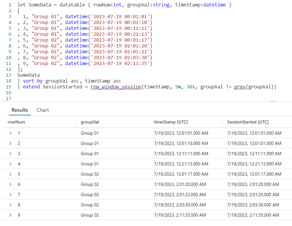
We begin by declaring a datatable to hold our sample data. It has three columns. The rowNum is included to make it easier to discuss the logic of row_window_session in a moment, otherwise it’s just an extra piece of data.

I then include a groupVal column. It will be used to trigger the beginning of a new time group (aka session). Working with real world data, you may use something like the name of a computer for the group.

Finally we have a column of datatype datetime. When working with log data from, for example, the Perf table this would typically be the TimeGenerated column but it doesn’t have to be. Any datetime datatype column can be used. I’ve crafted the data to make it easier to explain how row_window_session works.

Next, I take our SomeData dataset and pipe it into a sort, sorting by the group and time in ascending order. The sort has the added benefit of creating a dataset that is serializable. See my previous post on serialization, mentioned in the introduction, for more on why this is important.

Finally we fall into an extend where we create a new column I named SessionStarted. We then assign it the output of the row_session_started function, which requires four parameters.

The first parameter is the datetime column to be used for determining the session window. Here it is timeStamp. The next three parameters are all conditions which will trigger the beginning of a new “session” or grouping.

The second parameter is a timespan, here I used a value of 5m, or five minutes. If more than five minutes have elapsed since the current row and the first row in this group, it will trigger the creation of a new window session (group).

The third parameter is also a timespan, and indicates the maximum amount of time that can elapse between the current row and the previous row before a new window session is started. Here we used 30s, or thirty seconds. Even if the current row is still within a five minute window from the first row in the group, if the current row is more than thirty seconds in the future from the previous row a new session is created.

The final parameter is a way to trigger a change when the group changes. Here we use the groupVal column, but it’s more likely you’d use a computer name or performance counter here.

Breaking it Down

Since this can get a bit confusing, let’s step through the logic on a row by row basis. You can use the rowNum column for the row numbers.

Row 1 is the first row in our dataset, with a timeStamp of 12:01:01. Since it is first, KQL will use the same value in the SessionStarted column.

In row 2, we have a timeStamp of 12:01:10. Since this is less than five minutes from our first record, no new session is created.

Next, it compares the timeStamp from this row with the previous row, row 1. Less than 30 seconds have elapsed, so we are still in the same window session.

Finally it compares the groupVal with the one from row 1. Since the group is the same, no new session window is triggered and the SessionStarted time of 12:01:01, the time from row 1 is used.

Now let’s move to row 3. It has a time stamp of 12:11:11. This is more than five minutes since the time in row 1, which is the beginning of the session, so it then begins a new window session. It’s time of 12:11:11 is now used for the SessionStarted.

Row 4 comes next. It’s time of 12:21:13 also exceeds the five minute window since the start of the session created in row 3, so it begins a new session.

Now we move into row 5. Because the groupVal changed, we begin a new session with a new session start time of 12:01:17.

In row 6 we have a time of 02:01:20. Well a two am time is definitely more than five minutes from the row 5’s time, so a new session is started.

The time in row 7 is 02:01:22. That’s less than five minutes from row 6, and it’s also less than 30 seconds. Since it is in the same group, no new session occurs and it returns 02:01:20 for the SessionStarted.

Now we get to row 8. The time for this row is 02:03:30, so we are still in our five minute window that began in row 6. However, it is more than 30 seconds from row 7’s time of 02:01:22 so a new window session begins using row 8’s time of 02:03:30.

Finally we get to row 9. By now I’m sure you can figure out the logic. Its time of 02:11:35 is more than five minutes from the session start (begun in row 8), so it triggers a new session window.

Remember the Logic

While this seems a bit complex at times, if you just remember the logic it can be pretty easy to map out what you want.

Did the group change as defined in the fourth parameter? If yes, then start a new window session.

Compared to the session start row, is the time for the current row greater in the future by the value specified in parameter 2? Then start a new window session.

Compared to the previous row, is the time for the current row farther in the future then the amount of time in parameter 3? If so, start a new window session.

TimeSpans

In this example I used small values for the timespans, 5m and 30s. You can use any valid timespan though, including days and hours.

For a complete discussion on the concept of timespans, see my blog post Fun With KQL – Format_TimeSpan.

Let’s Use Real Data

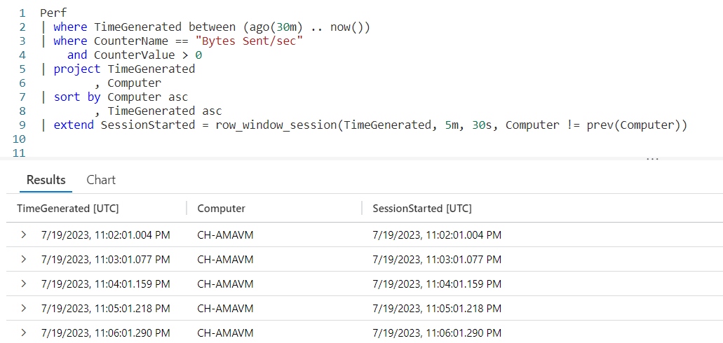
For completeness I wanted to include a final example that uses the Perf table from the LogAnalytics demo website.

The logic is similar to the previous example. Since you now have an understanding of the way row_window_session works, I’ll leave it up to you to step through the data and identify the new window sessions.

Conclusion

With this post on row_window_session, we complete our coverage of Kusto’s Windowing Functions. You saw how to use it to group data into timespans based on a beginning date, with the ability to group on total elapsed time since the start of a window or since the previous row of data.

The demos in this series of blog posts were inspired by my Pluralsight courses on the Kusto Query Language, part of their Kusto Learning Path.

There are three courses in this series so far:

I have two previous Kusto courses on Pluralsight as well. They are older courses but still valid.

These are a few of the many courses I have on Pluralsight. All of my courses are linked on my About Me page.

If you don’t have a Pluralsight subscription, just go to my list of courses on Pluralsight. On the page is a Try For Free button you can use to get a free 10 day subscription to Pluralsight, with which you can watch my courses, or any other course on the site.

Fun With KQL Windowing Functions – Row_Rank_Dense

Introduction

The Kusto Windowing Function row_rank_dense is an interesting function. It lets you get a unique count of a specific column in a dataset. Unlike other methods of getting counts, row_rank_dense allows you to see each individual row of data.

First though, if you’ve not read the introductory post on Windowing Functions, Fun With KQL Windowing Functions – Serialize and Row_Number, you should do so now as it introduced several important concepts needed to understand how these Windowing Functions work.

Row_Rank_Dense Basics

The row_rank_dense is used to determine the density of a value. By passing in a sorted dataset, you can get a rank number for each item. The rank number changes only when the value we’re evaluating changes.

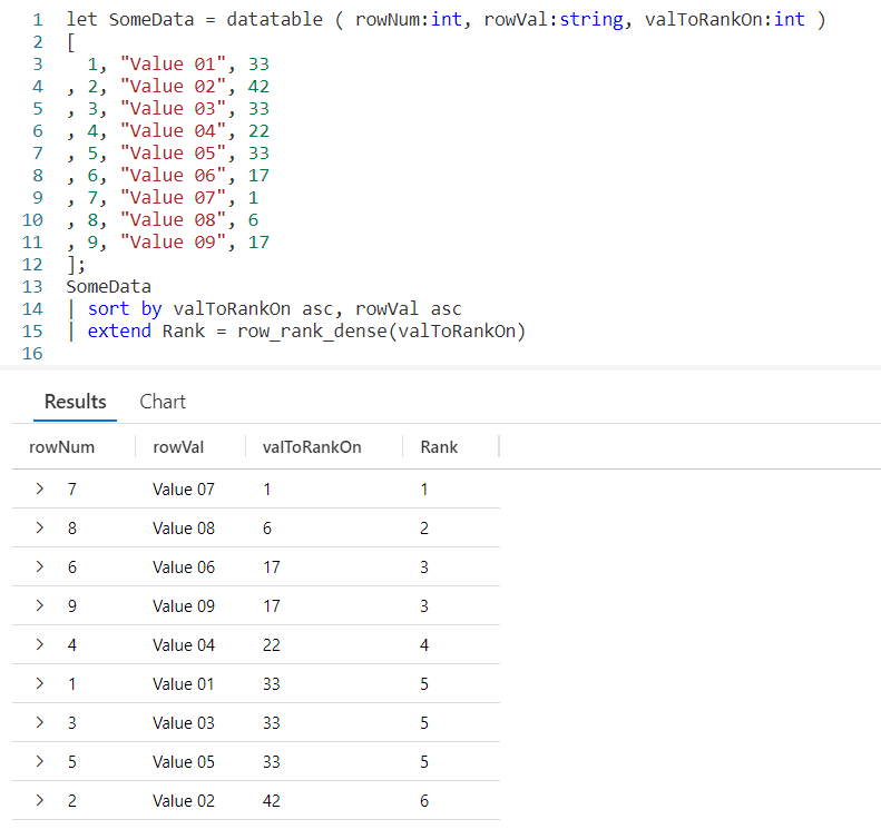
An example will make this much clearer. We start by creating a datatable with three columns. The rowNum is just used to make it easier to discuss the output in a moment. Likewise rowVal provides some easy to consume text.

The important column is valToRankOn. It is this value that is going to be evaluated within our row_rank_dense Windowing Function.

The SomeData dataset is piped into a sort, where we sort on the value we are evaluating in ascending order. We will also sort on the rowVal, so when we have two identical values in valToRankOn, we can display the output in a logical fashion. In a real world situation, this might be the name of computer or perhaps a counter of some kind.

Using a sort will also mark the data as serializable, which is required in order to use row_rank_dense. For more on serialization, see the Fun With KQL Windowing Functions – Serialize and Row_Number post I mentioned in the introduction.

Finally we fall into an extend, creating a new column Rank. We’ll assign it the output of our row_rank_dense function. In it we use one parameter, the name of the column to be evaluated, here it is valToRankOn.

In the output, our first row is row 7, with a valToRankOn of 1. Thus it is assigned a Rank of 1.

The next row is row 8, it has the next smallest value of 6 in the valToRankOn column, so it gets a Rank of 2.

Rows 6 and 9 both have the same valToRankOn, 17. Since 17 is the third smallest value, both rows are given a Rank of 3. Because we included rowVal in the sort, they are listed in order of the rowVal, Value 06 then Value 09.

This continues for the remaining rows of data. We can see both how many unique values we have, six, and still see each individual row of data.

Density by Largest Value

In the above example, by sorting the valToRankOn in ascending order the smallest values come first, then increase with a Rank of 1 being given to the smallest value.

If we had instead sorted valToRankOn in descending order, sort by valToRankOn desc, ..., then the Rank of 1 would have been assigned to the largest value, then as the valToRankOn decreased the Rank would have increased. I’ll leave it as an exercise for you to play with this by altering the sort order for your sample queries.

Grouping In Row_Rank_Dense

It is also possible to organize rankings within a group. For example, within a single computer you might want to rank a counter value. With the next computer you’d want the rankings to begin again. This would allow you to have rankings that are unique to each computer.

In the example below I’ve added a new column to the datatable named groupVal. We’ll be using this column for our grouping. It was also added to the sort operator so we’ll sort by group first, then the value to rank on, and finally the rowVal text.

The row_rank_dense function supports a second parameter, a boolean value that when true will trigger a new group to begin. Here we are using an equation, which will compare the groupVal for the current row to the one of the previous row using the prev Windowing Function. If they are not equal, the comparison will return true and trigger row_rank_dense to begin a new dense rank grouping.

In the output, rows 1 and 3 (from the rowNum column) have the same valToRankOn, so are both given the Rank of 1. The third row in this group, row 2, is assigned a Rank of 2.

With row 4, we see the groupVal has changed. So the row_rank_dense function reset and began a new ranking, assigning this row a Rank of 1.

When the group changes again in row 7, the Rank value is again reset to 1 and we work our way up.

Row_Rank_Dense in the Real World

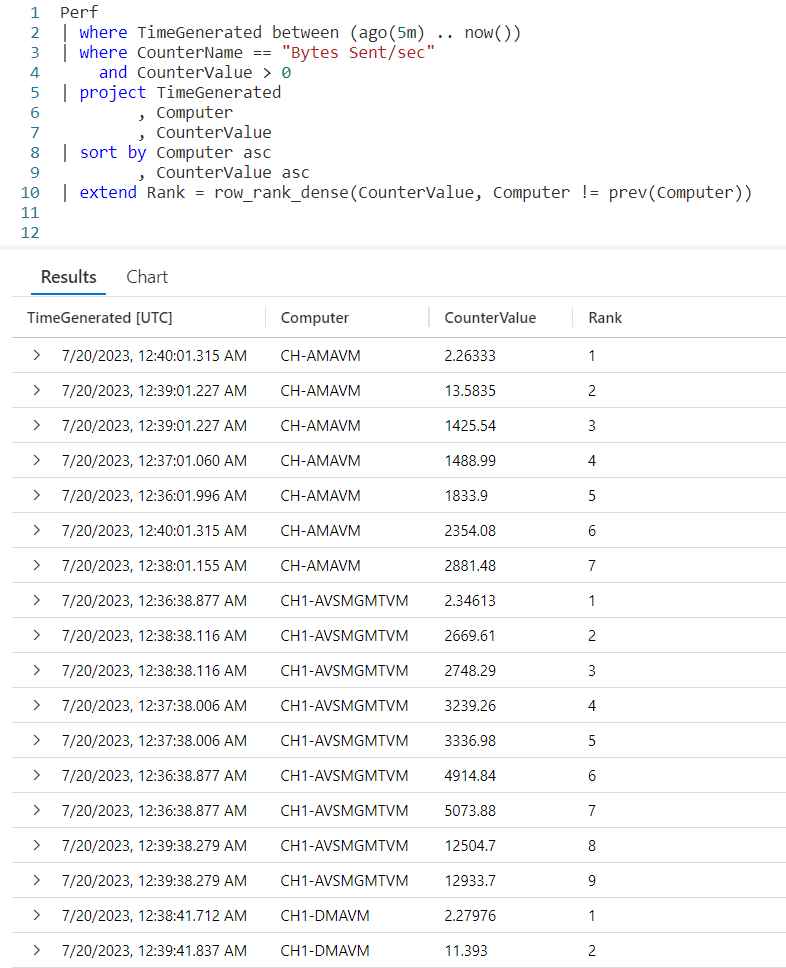
Let’s take a look now at an example of using row_rank_dense for a “real world” query. Here, we are going to query the Perf table to bring back rows for the last five minutes where the CounterValue is Bytes Sent/sec, and we’ll remove any rows with a value of zero.

We’ll project each column we need and sort the data. Here we’ll again sort in ascending order so the smallest counter values come first, but we could just have easily sorted the CounterValue in descending order so the largest values came first.

When we call row_rank_dense, we’ll pass in the value we want to rank in the first parameter, CounterValue. In the second parameter we’ll compare the name of the computer in this row to the one of the previous row using the prev function. When they don’t match the comparison will return true, which will trigger the row_rank_dense function to begin a new group.

As you can see, we begin with computer CH-AMAVM, with its value of 2.26333 given the rank of 1, then the rank values increase as the counter values increase.

When we hit computer CH1-AVSMGMTVM, note the Rank reset itself. The first row for this computer, with a counter value of 2.34613 has a Rank of 1.

This pattern will repeat for the remaining rows of data from our query.

Conclusion

In this post you saw how to use the row_rank_dense Windowing Function to order and rank values in a dataset from smallest to largest, or largest to smallest.

The next and final post in the Kusto Window Functions series will cover the use of row_window_session to group and organize data into time windows.

The demos in this series of blog posts were inspired by my Pluralsight courses on the Kusto Query Language, part of their Kusto Learning Path.

There are three courses in this series so far:

I have two previous Kusto courses on Pluralsight as well. They are older courses but still valid.

These are a few of the many courses I have on Pluralsight. All of my courses are linked on my About Me page.

Fun With KQL Windowing Functions – Row_Rank_Min

Introduction

In this post we’ll cover the next in our series on KQL Windowing Functions, row_rank_min. The row_rank_min function will assign rank numbers to an incoming dataset, with the rank of 1 being assigned to the minimal value in the dataset and increasing as the values increase.

Row_Rank_Min Basics

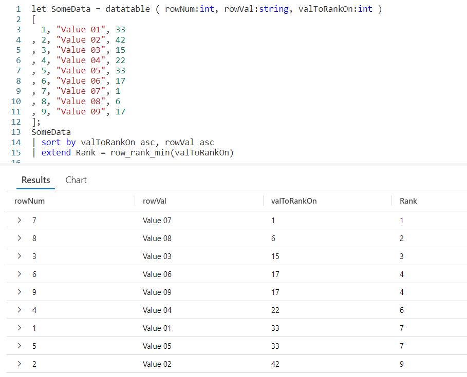
We being by using let to define a datatable with some values to use for our example. The rowNum and rowVal are just included to have some data to look at.

The important column is valToRankOn. This is the column that will be evaluated and used to rank the data. Let’s see how our query works.

We take our SomeData and pipe it into a sort, sorting by the value to rank on and the row value (rowVal). Note we need to sort the valToRankOn in ascending order to get the row_rank_min to work correctly, and while we are at it we’ll sort the rowVal in ascending order as well.

The sort has the added benefit as making the data serializable, so it can be used with KQL Windowing Functions, in this case row_rank_min. For more on serialization see the post I referenced in the introduction, Fun With KQL Windowing Functions – Serialize and Row_Number.

After the sort we have an extend where we create a new column Rank. To it we assign the output of row_rank_min. Into the function we pass the column to evaluate for the rank, here we are using valToRankOn.

The smallest value is given a rank of 1, as you can see with rowNum 7. The next smallest value, found on rowNum 8 is assigned a rank of 2. Row 3 has a valToRankOn of 15, which is the next smallest value so it was given a rank of 3.

Rows 6 and 9 both have a value of 17, so both are assigned the same minimal rank number of 4. Because we added the rowVal to the sort, the rows are sorted in ascending order by the rowVal within the Rank of 4.

This pattern is repeated for the remaining rows, with the rank value increasing as the values in valToRankOn increases. As you can see, this provides an easy way to rank values from smallest to largest.

Ranking Within a Group

Similar to the row_cumsum Windowing Function we looked at in the previous post, we can create rankings within a group. In the following sample, a new column of groupVal was added to the SomeData sample dataset.

In the example we made two changes from the previous sample. First, the groupVal was added to the sort statement.

The next change occurred in the row_rank_min function. It supports a second parameter that will trigger a reset of the ranking value. It needs to evaluate to a boolean true/false value. When true, it resets the ranking value.

Here, we are comparing the groupVal of the current row to the groupVal of the previous row using the prev function. If the group name for the current row is different from the previous row, the comparison will return true since they are not equal. This will trigger the ranking to restart.

In rowNum 4 the group changes to Group 2, so Kusto starts the ranking again. Within Group 2, the value of 22 on row 4 is the smallest, so it gets the rank of 1.

This technique lets us create minimal ranking values within individual groups of data. Here we are using groupVal, in a real world you might use something like a computer name or performance counter name.

Real World Example

In this query we’ll create something you might use in the “real world”. We’re going to look at the Perf table for the counter “Bytes Sent/rec”, where there is data (the counter value is greater than zero).

We’ll project only the columns we need, then sort the output. We want to create rankings for each computer, from the smallest counter value to the biggest. By doing so we can easily see what times we had the smallest and largest values.

Here we use row_rank_min to evaluate the CounterValue. In the second parameter we are checking to see if the Computer name has changed, if so the rank will reset for the next computer.

Looking at one example, when the Computer changed from CH-AMAVM changes to CH1-AVSMGMTVM, the rank reset so the smallest value of 16.4175 is given the rank of 1.

Conclusion

With this post we saw how to create rankings for values using the row_rank_min function. This allows us to easily identify the smallest value, with a rank of 1 and work up to the largest value.

In our next post we’ll continue our KQL Windowing Function series by looking at the row_rank_dense function, which is similar to this posts row_rank_min.

The demos in this series of blog posts were inspired by my Pluralsight courses on the Kusto Query Language, part of their Kusto Learning Path.

There are three courses in this series so far:

I have two previous Kusto courses on Pluralsight as well. They are older courses but still valid.

These are a few of the many courses I have on Pluralsight. All of my courses are linked on my About Me page.

Fun With KQL Windowing Functions – Row_CumSum

Introduction

Seeing cumulative totals on a row by row basis is a common need. Think of your bank account, when you look at your ledger it shows each individual transaction. Beside each individual transaction is the current amount in your account, as offset by the amount of the current transaction.

This technique is known as cumulative sums. The Kusto Query Language provides the ability to create cumulative sums using the Windowing Function, row_cumsum. In this post we’ll see how to implement it.

If you’ve not read my introductory post in this KQL series, I’d advise you to do so now. It describes the user interface in detail. You’ll find it at https://arcanecode.com/2022/04/11/fun-with-kql-the-kusto-query-language/.

Row_CumSum Basics

For this example I’ll be using let to generate a simple dataset using the datatable operator. It will have two columns, the row number rowNum, and a value rowVal. For more information on let, datatable, serialize, and other functions used in this post refer to the See Also later in this post.

Using row_cumsum is simple. First, we need to pipe the dataset SomeData into a serialize so we can use it with Windowing Functions. The serialize also lets us create a new column we named cumSum, and set it equal to the row_cumsum output. As a parameter, I pass in the numeric column I want to add up, here I used the rowNum column.

As you can see in row 1, the row number (rowNum) has a value of 1. There is no data since there are no previous rows, so it just returns 1.

In the second row, the value of rowNum is 2. The cumSum column already had a value of 1, so we’ll add 2 to it, for a result of 3.

With the third row, we’ll add the value in rowNum (3) to the value in cumSum (which also happened to be 3) and we’ll now have a cumulative sum of 6.

This repeats for each row, creating a cumulative summary.

You can also create a way to decrement the data by using a negative value for the row_cumsum parameter. For example, row_cumsum(rowNum * -1) could have been used to create a decrementing value much as spending money out of your checking account would decrement your balance. You’d just want to determine the best way to handle the beginning value (first row) of the dataset.

Resetting the Cumulative Counter

It’s possible you may not want to keep accumulating for all rows, but instead only have the accumulation for a group of rows. A common task is to reset the sum when a computer name changes, or perhaps the calendar month.

For this example, I’ve added a third column to our datatable, rowBucket. Whenever the value in rowBucket changes, I want to reset the cumulative sum value.

The row_cumsum supports a second parameter that is a boolean value. When true, the counter resets. Here, I’m using an equation to calculate “is the current rows rowBucket value not equal to the one from the previous row”. If this is true, in other words not equal, then the counter will reset.

Sure enough, on row 4 the rowBucket changed to 2. On this row the cumulative sum reset itself. It now keeps adding up until the bucket number changes again, as it does with row 6.

A Real World Example

Using a datatable made the examples easy to understand, but it’s time to look at an example you might want to use in the “real world”.

Let’s imagine a scenario where you’ve detected a large amount of network traffic coming from one of the computers on your Azure network. You’d like to check the performance log table (Perf) to see how many bytes each computer sent in the last five minutes.

You need to see the number of bytes sent by a computer for each log entry, but you also want to see the total bytes sent by a computer for that time period. Let’s look at a query to accomplish this goal.

We begin with our old buddy the Perf table. A where will limit the data to the last five minutes. A second where will limit the counter to just the one we are interested in, Bytes Sent/sec. Since we only need to see this data when the virtual Azure server sent data, we’ll add a final where to remove any rows where the CounterValue is zero.

Next, we’ll use a project to strip down the columns to only the three we are interested in: the Computer, TimeGenerated, and CounterValue.

We then want to use a sort, so the data for each computer will be grouped together, then within a Computer the time the performance data was generated. Note that since the default for a sort is descending order, an asc was added after the TimeGenerated so the entries would go from the oldest to the most recent.

I normally might include an asc after the Computer so the computer names would be sorted alphabetically from A to Z, but left it off for this example just to remind you that with a sort you can mix and match the asc and desc columns.

Using a sort has another benefit. If you did go back and read my post Fun With KQL Windowing Functions – Serialize and Row_Number as I suggested in the introduction, you’ll know that the sort marks a dataset as safe for serialzation. In order to use Windowing Functions, such as row_cumsum and prev, a dataset needs to be safe for serialization.

The final line of the query is where the magic happens. Since using sort eliminated the need to use serialize, we can just use an extend to create a new column. I chose to name it cumulativeBytes.

We assign it the output of our row_cumsum Windowing Function. In the first parameter we pass in the CounterValue. In the second column we create an expression that will evaluate to true or false. We compare the Computer column for the current row and call the prev Windowing Function to get the Computer from the previous row of data.

If they are not equal, then the equation returns true. This will cause the row_cumsum to reset the cumulative sum.

Looking at the output, you can indeed see that occurred. The first computer in the list is CH1-VM-CTS. With each row it begins accumulating the CounterValue into the cumulativeBytes column.

When the Computer changed to CH-DMAVM, you can see the cumulativeBytes counter was reset. It kept accumulating the values for CH-DMAVM until the Computer changed to CH-AVSMGMTVM at which point it was again reset, and the pattern continues.

Conclusion

Cumulative sums are not an uncommon need when retrieving data. Kusto provides this ability with the Windowing Function row_cumsum, which you saw how to use in this post.

Our next post will continue the coverage of Kusto Windowing Functions by looking at the row_rank_min function.

The demos in this series of blog posts were inspired by my Pluralsight courses on the Kusto Query Language, part of their Kusto Learning Path.

There are three courses in this series so far:

I have two previous Kusto courses on Pluralsight as well. They are older courses but still valid.

These are a few of the many courses I have on Pluralsight. All of my courses are linked on my About Me page.

Fun With KQL Windowing Functions – Prev and Next

Introduction

In this post we’ll continue our series on Kusto’s Windowing Functions by covering prev and next. If you’ve not read the introductory post, Fun With KQL Windowing Functions – Serialize and Row_Number, you should do so now as it introduced several important concepts needed to understand how these functions are used.

So what do prev and next do? They allow you to retrieve a value in a column from a previous row, or the next (or upcoming) row. This can be very useful in many situations. For instance, calculating the time between two rows based on a datetime column, or the change in a value from one row to the next.

Prev Basics

To make these examples simple, I’m going to use the datatable operator to generate a very simple dataset. For more on how datatable works, please see my post Fun With KQL – Datatable.

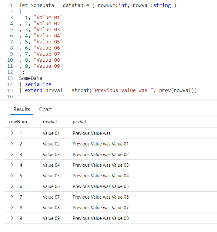
Using a let, I’ve created a dataset named SomeData. It has nine rows and two columns: rowNum and rowVal.

After my let, I take the SomeData dataset and pipe it into a serialize so it can be used with Windowing Functions like prev. Refer back to my previous post on serialize for more information on how serializing a dataset lets you use Windowing Functions.

Now the data pipes into an extend, where we add a new column I named prvVal (short for previous value). We then use strcat to combine a text string, Previous Value was with the output of our prev Windowing Function.

Into prev we pass one parameter, the name of the column from the previous row we want the data for. Here we want to pull data from the column rowVal.

As you can see in the output, the right most column displays our Previous Value was text string, plus the value from the rowVal column in the previous row.

Even More Previous

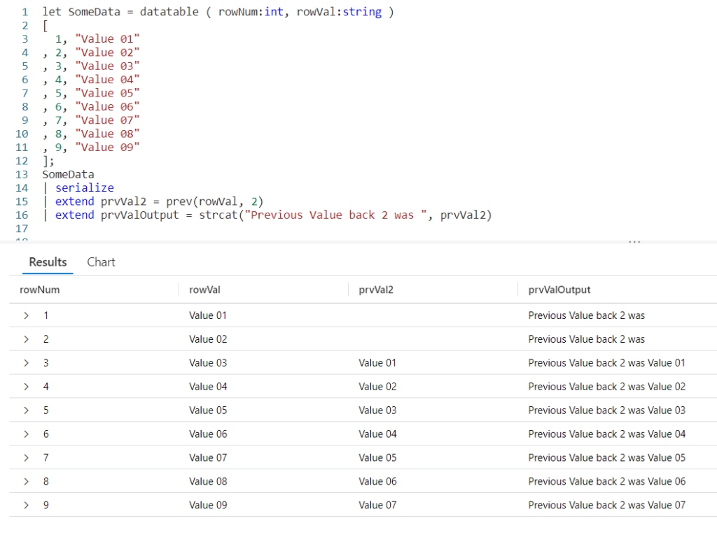
We can go back more than just one row. The prev function supports a second parameter that indicates the number of rows to go back.

First, I decided to use two extends. The first will copy the previous value into a variable, prvVal2. Into the prev function I pass two values, the first is the column name we want the data from. Here we’ll use rowVal again. The second parameter is the number of rows we want to go back, in this case we just used the value of 2.

In the next extend I user strcat to combine the prvVal2 variable with a text string and put it into the new column prvValOutput. I did this just to demonstrate you could pull a value from a previous row and use it in the query. I could have done other things with prvVal2, such as use it in a calculation.

Previous Value? What Previous Value?

You probably noticed that when we are on the first row, there is no previous value. Likewise, when on the first or second rows, and going back two there was no data. In this case the prev just returned a null value.

In the past I’ve written about functions like iif and isnull to help handle null values. Fortunately, prev eliminates the need for these as it supports and optional third parameter. Into it you can supply a value to use when the value returned by prev would otherwise be null.

In our prev we first pass the column from the previous row we want the data from, rowVal. In this example we are only going to go back one row, but since we want to use the third parameter we have to supply a value in the second parameter position. In this example we’ll use the number 1.

Finally in our third parameter we supply a value to be returned when the result of a prev would be null. Here we used the text not valid for this row, although we could have used a different datatype such as a numeric value or a datetime if that would have been more appropriate to our query.

Next, let’s look at next. The next function behaves just like prev, except it will get data from the next row in our serialized dataset instead of a previous row.

Just like with prev, as the parameter to next we pass in the name of the column to get the data from.

The next function also supports the optional second and third parameters. The second being a number indicating how many rows to go forward, the third being a value to use when next would otherwise return a null value.

Since you’ve already seen these in play I won’t create samples here, but you should be able to easily create them for yourself following the examples from prev.

Calculating a Moving Average

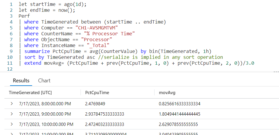
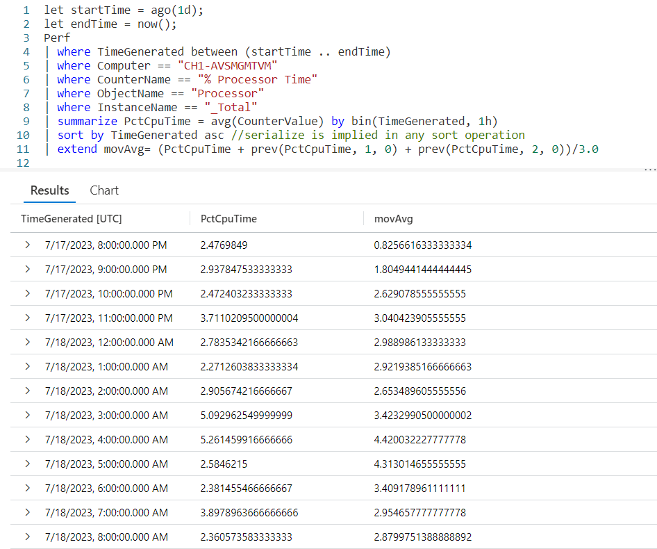
So it’s time for a more realistic example. Here I want to get the % Processor Time from the Perf table for a particular computer. I’m going to summarize it by hour. Then I want to create a moving average for the last three hours.

Most of the query will be pretty straightforward if you’ve been following my KQL series. I capture a start and end time using let. I then use the Perf table, followed by several where statements to limit the data.

Next I use summarize to create an average, bucketed by hour. In essence I’ll have an average of all the processor times for the 1 am hour, then 2 am, and so on.

After that we’ll sort them by the time of the day. Not only will the sort put the data in the order we want, it will also mark them as serialized. This means we can use them with our Window Function prev.

The last line is where the exciting things happen, so take a look and we’ll break it down.

We begin with extend in order to create a new column, movAvg. We are then going to add three values. The first value is the PctCpuTime from the current row, which was calculated during the summarize.

Next, I want to add in the PctCpuTime from the previous row. To do that we’ll use the prev function, pass in the PctCpuTime as the column to get, 1 to indicate we want to go back one row, then tell it to return a 0 (zero) when the previous row would return null.

This is then repeated only we pass in a value of 2, indicating we should go back two rows.

After the closing parentheses we divide by 3.0. Note its important to include the .0 otherwise it would try to create an integer output and we want a full decimal value.

And there you go, we now have an average for the last three rows of data.

Let me acknowledge, by returning a 0 for missing (null) values from the prev, the averages for the first two rows will be off. In a real world situation you’d want to make sure to take this into account, creating a solution appropriate to your situation. For this example I used zero in order to keep things simple.

Conclusion

This post continued our journey with KQL Windowing Functions, seeing how the useful prev and next functions could get data from adjacent rows of a serialized dataset. In our next post we’ll be looking at a Windowing Function to let us get cumulative sums.

The demos in this series of blog posts were inspired by my Pluralsight courses on the Kusto Query Language, part of their Kusto Learning Path.

There are three courses in this series so far:

I have two previous Kusto courses on Pluralsight as well. They are older courses but still valid.

These are a few of the many courses I have on Pluralsight. All of my courses are linked on my About Me page.

Fun With KQL – New Pluralsight Course! Kusto Query Language: Scalar Operators

Introduction

My third course in the Pluralsight Kusto Query Language Learning Path has just been published: Kusto Query Language: Scalar Operators. This course is the third in Pluralsight’s Kusto Query Language Learning Path.

The Kusto Query Language has a rich set of scalar operators. Operators that can be used to transform your data, making the output of your queries easier to read.

In this course, we cover some of the most used Kusto Query Language scalar operators, which will enable you to author effective queries right away.

Some of the major topics that are covered include:

Work with dates and times, including datetime math as well as formatting.
Logic branching
Working with strings
Advanced techniques for working with column data

By the end of the course, you’ll have enough information about scalar operators to write queries with more readable output.

Kusto Query Language: Previous Courses

If you have not seen my previous two courses in the series, you should probably watch those first if you are not familiar with KQL.

The first course, Kusto Query Language: Getting Started, covered the basics of KQL, as well as the user interface.

In the second Pluralsight course, Kusto Query Language: Beginning Operators, I cover some of the most useful of the KQL operators. Using this course you can write effective queries in order to do most of your data retrieval.

The newest course, which I mentioned above, shows how to take your output and format it nicely for a wider audience.

No Pluralsight Subscription? No Problem!

Every good IT organization should have a place for it’s staff to continue their education, and stay up to date with the latest IT subjects. Pluralsight is a great choice, it can be done on demand, has a HUGE catalog of courses, is constantly being updated, and the courses are done by leading IT professionals.

Talk to your boss about it, you’d be amazed at how many things you can get in life just by asking (using a persuasive argument of course).

While waiting for your organization to get approval, there is a way to watch for free. Just go to my list of courses on Pluralsight . At the top is a Try For Free button you can use to get a free 10 day subscription to Pluralsight, with which you can watch my courses, or any other course on the site.

Conclusion

Just a side note for those who subscribe to my posts. Normally I publish on Mondays, but this post was a bit late this week due to wrapping up the course. I’ll probably take next week off of my KQL series and resume the week after.

I hope you enjoy the courses! And stay tuned to the blog, as I will be continuing my ongoing series Fun With KQL.

Fun With KQL – Let

Let me tell you about let, my favorite operator in the Kusto Query Language. Why my favorite?

It is extremely flexible. It lets you create constants, variables, datasets, and even reusable functions. Let me tell you, it’s very powerful.

Before I go further, let me say the samples in this post will be run inside the LogAnalytics demo site found at https://aka.ms/LADemo. This demo site has been provided by Microsoft and can be used to learn the Kusto Query Language at no cost to you.

A Quick Note on Casing

If you have been following my posts in this Fun With KQL series, you’ll have noticed that operators and functions in KQL are all in lowercase. Table and column names though are almost always in mixedcase, although when users create their own data clusters they can use whatever casing they wish. In mixed case, the first letter is capitalized, then letters of distinct words are also capitalized. Some examples are Perf, AppRequests, and AppAvailabilityResults.

As mentioned in the intro, let allows you to create variables to hold variable data, constants, and functions. To keep these distinct from other KQL items I use what is known as camel case. With camel casing, the first letter is in lower case, but any different words after it are placed in capitals. Some examples you’ll find later in this post are timeDiffInDays, usageData, and counterName.

Using camel case immediately lets me identify a name as being created from a let statement and not an operator or table / column name. The use of camel case is not a requirement, but it is a common practice among many of us who use the Kusto Query Language.

Using Let to Create a Constant Value

Using let in its most basic form is very simple. You simply use let, followed by the name of the variable you want to create. Next comes an equal sign, and the value you want to assign to it. The let must end in a semicolon (;).

You can have multiple let statements before your query, as you see in this example. Then within the main query, you use the variable name as you would any column name, table or operator.

Here, we set two variables, minCounterValue and counterName. Placing these values in constants like we do makes them easier to change between runs of the query. For example, perhaps the first time we run the query it returns too many rows, so we can easily change the minimum counter value to say 100 to reduce the number of rows we will need to work with.

This is especially useful when we use the values in multiple places in the query. Here they are used in the strcat operator. Then, they are both used in the where operator. This is a simple query, but you can see how useful it is to be able to quickly change values in one quick setting.

Allow me to point out one other thing, a reminder really, that Kusto is case sensitive. CounterName is a different object than counterName. It is this case sensitivity that allowed us to use where CounterName == counterName in our query.

Be careful when doing this, sometimes it’s too easy to miss the difference in casing when quickly looking over a query. For that reason I suggest avoiding situations such as using CounterName and counterName in the same query. I did it here so I could demonstrate the concepts.

Using Let to Create a Calculated Value

You can also use let to create a value based on a calculation. Here we are doing something very simple, and setting the startDate to twelve hours ago. This makes it very easy for us to alter the calculated value between executions of the query.

Of course you could create far more complex calculations, I kept it simple for this demo.

Also keep in mind, at the time the let statement executes, the main query has not yet executed. Thus you won’t have access to any of the columns in your query.

There’s a way around this though, through the use of functions which we’ll see in the next section.

Creating a Reusable Function with Let

If you want to create a reusable calculation, but need to work with data from your dataset, you’ll need to create a function.

We start by creating the name of the function then an equal sign: let timeDiffInSeconds = .

Next we have parenthesis that enclose the list of parameters we want to use. You can have as many parameters as you need, or none at at all. In our function we need two.

For each parameter we need to indicate the name we want to use inside the function, then a colon, and the datatype for the parameter.

Here we named the parameters date1 and date2, then the colon followed by the datatype. In this case we specified datetime for both of them: (date1: datetime, date2: datetime).

Following the list of parameters we then define the function. The function is enclosed in squiggly braces { }. The function is pretty simple, we take the date2 parameter and subtract the date1 parameter. The result is divided by one second, so the time difference will be returned in seconds: { (date2 - date1) / 1s }.

Here we could fit our function into a single line, but you can use any number of lines you need as long as it is still valid code. For example we could have done:

{
  (
    date2 - date1
  )
  / 1s
}

To be honest this is an example that makes the code a lot harder to read, and if you ever see production code from me that looks like this it’s a clear indicator I’ve been kidnapped by space aliens and am asking for help. But here, it serves to illustrate the point that my function can spread out over multiple lines.

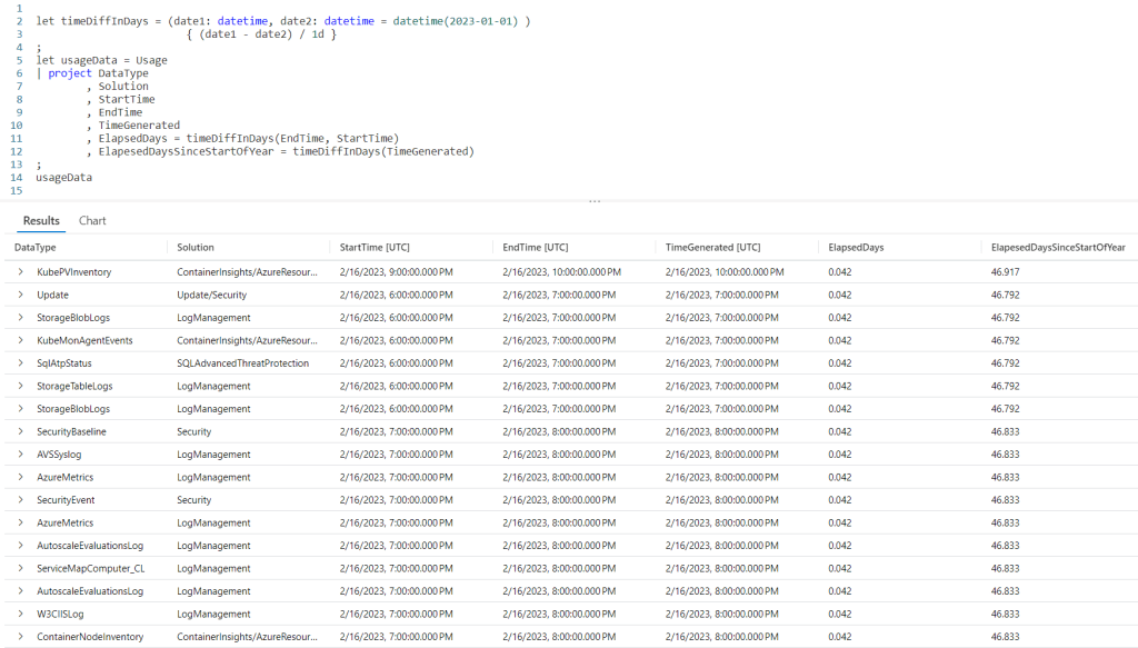
Using the let defined function is simple. In the project we simply create a new column name, ElapsedSeconds and assign to it the function we created in the let, here timeDiffInSeconds. As parameters we then pass in the StartTime and EndTime. This results in:

ElapsedSeconds - timeDiffInSeconds(StartTime, EndTime)

Here it is in action.

As you can see in the output, we have our ElapsedSeconds column which shows the difference in seconds between the start and end times.

Functions with Default Values

It’s also possible to supply a default value for the last parameter in your list. Before I go on, let me warn you this is an undocumented feature. The online help for the let statement makes no mention of defaults, so USE THIS AT YOUR OWN RISK. I cannot predict how Microsoft may alter this feature in the future.

I discovered this when I created the first version of the Kusto course for Pluralsight around 2018. For it I was working closely with Microsoft on the content and it was included in the samples they wanted to use. I’m not sure why it is now undocumented, they may plan to discontinue, or change its behavior. So let me say one more time, use at your own risk.

In the list of parameters after the datatype for the last parameter we use an equal sign, followed by the default value.

In this example, if we do not pass in a value for the second parameter it uses the default value supplied. Here, date2: datetime = datetime(2023-01-01) will return January first of 2023 when no date is supplied.

For this example we also altered the function to return the time difference in days instead of seconds.

Looking at the last line of the query, you can see we used ElapesedDaysSinceStartOfYear = timeDiffInDays(TimeGenerated) and only passed in one value, the TimeGenerated.

Right above that we had a line, ElapsedDays = timeDiffInDays(EndTime, StartTime). In this line we passed in two values. Instead of using the default it instead used the value in StartTime. This gave our function a lot of flexibility.

Note default values do have one issue, you can’t use dynamic values such as ago(20d). That’s why we needed to hard code the January first date.

Creating Useful Functions

Back in my post Fun With KQL – Case, I showed how to use a case statement to retrieve the name of the month based on the month number that was used.

This is a useful piece of code, so I created a function out of it. I have a file full of these useful pieces of code. Putting them in functions makes them easy to reuse.

In this function I simply create one parameter, the monthNumber. It will return the text associated with the month number passed in. For more on how the case works, refer back to my Fun With KQL – Case post.

I then added a second useful function, getNiceDate, which uses string concatenation to assemble a nice date. For more on the strcat and format_datetime operators see the See Also section of this post for links to the associated blog posts I’ve done.

In my query I used a couple of extends to call my functions then add their output to my query. I could have done away with the extends and just embedded the calls the functions right inside my project. I just thought separating it out made it a little easier to read.

As you can see in the output, I have both the MonthName and NiceDate columns with the nicely formatted data.

Using a Let to Hold a Dataset

The let operator can also hold a dataset, often referred to as a datatable in Kusto.

In the second let statement, I simply provide a name to hold the dataset, here usageData. I then supply the query needed to get the data.

In the final line I simply use the variable usageData to send the data to the output pane.

Right now this may not seem very useful, but in upcoming posts on join and union you’ll see how to use this functionality. For now just remember it as it will prove useful soon.

Conclusion

In this post we explored the versatile let operator. We first saw how to use let to hold constant values. Next we learned how to hold variables using let.

From there we saw how to create reusable functions, in my humble opinion lets greatest power. Finally we saw how to use let to hold a dataset, also called a datatable. We’ll explore this last capability more in upcoming blog posts.

The demos in this series of blog posts were inspired by my Pluralsight courses on the Kusto Query Language, part of their Kusto Learning Path.

The first course in the series is Kusto Query Language: Getting Started. The second course is Kusto Query Language: Beginning Operators. The third course, to be published soon, is Kusto Query Language: Basic Scalar Operators

I have two previous Kusto courses on Pluralsight as well. Kusto Query Language (KQL) from Scratch and Introduction to the Azure Data Migration Service, and these are two of the many courses I have on Pluralsight. All of my courses are linked on my About Me page.

If you don’t have a Pluralsight subscription, just go to my list of courses on Pluralsight . At the top is a Try For Free button you can use to get a free 10 day subscription to Pluralsight, with which you can watch my courses, or any other course on the site.

Fun With KQL – Take_Any

Introduction

The take_any function is a random row generator. Based on the parameters passed it, it will select a random row from the dataset being piped into it. It also has a variant, take_anyif, we’ll see both in this post.

Note that take_any was originally called any and was renamed. While any still works, it has been deprecated and you should now use take_any.

Any and all of the samples in this post will be run inside the LogAnalytics demo site found at https://aka.ms/LADemo. This demo site has been provided by Microsoft and can be used to learn the Kusto Query Language at no cost to you.

Take_Any Basics

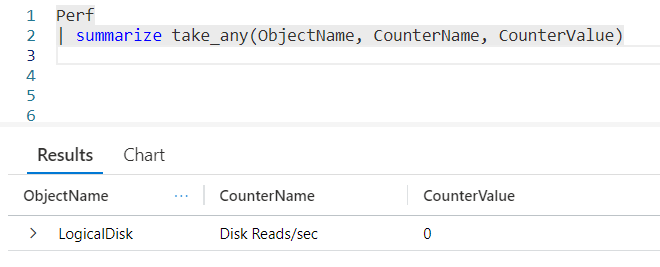
Like other functions we’ve covered so far, we will need to use summarize in order to execute take_any. In this example, we will pass an * (asterisk) into the take_any parameter. This will cause all columns for a random row to be returned.

Each time you execute this you should get a different row back from the piped in dataset. Note there are more columns that appear off screen to the right.

Take_Any For A Column

With take_any, you can also pass in a specific column name instead of using the *.

As you can see, it returns a random value from the column passed as the parameter.

Take_Any With Multiple Columns

take_any can also work with multiple columns. Just pass each column you want as a parameter, and it will return the values from a random row that contains the columns you requested.

Here, we passed three columns from the Perf table into take_any. It returned a random row with the three columns. We could have used more columns or less, according to our needs.

Returning Random Multiple Rows Based On A Column with Take_Any

You can return multiple rows from take_any. To do so, you can add by then the column name after the take_any as you can see in this example.

Here we passed an * to get all columns, then we follow with by CounterName. KQL will get a list of unique CounterNames then return a random row for each one.

Take_AnyIf

The take_anyif variant of take_any operates like other if variants we covered recently, maxif, minif, and sumif.

We pass in the name of a column in the first parameter, then the second parameter is a condition. In this case, the row that will be picked randomly must have a CounterName of % Free Space.

In the results, you can see it grabbed a random computer name from the Computer column where the CounterName for that row had a value of % Free Space.

take_anyif does have a few limitations compared to take_any. First, you cannot pass in an * and get all columns. Second, you can only enter a single column. It does not support passing in multiple columns.

Conclusion

In this post we learned how to use take_any to grab a random row. We saw how to return all columns, a single column, or multiple columns. In addition we saw how to use take_anyif to grab a random value conditionally.

The demos in this series of blog posts were inspired by my Pluralsight courses on the Kusto Query Language, part of their Kusto Learning Path.

Fun With KQL – Sum and SumIf

Introduction

In my previous post, Fun With KQL – Max, MaxIf, Min and MinIf, we looked at the aggregation functions max and min. In this post we’ll talk about another aggregation function, sum. We’ll also look at a variant of it, sumif.

I should mention the samples in this post will be run inside the LogAnalytics demo site found at https://aka.ms/LADemo. This demo site has been provided by Microsoft and can be used to learn the Kusto Query Language at no cost to you.

Sum Basics

The sum function is straightforward. It creates a total for the column passed into it.

In this demo we’ll take the Perf table, and filter it with a where operator to only include rows where the CounterName is Free Megabytes.

We then call summarize, which is needed if you want to use an aggregation function on its own. Finally we use sum and pass in the column we want to total, CounterValue.

In this example, we result in a total of 6,398,287,032.

Including the Sum As A Column

We can include the sum function as a column in the output. To do so we need to include a by as part of the summarize so the data will be grouped correctly, in this case by the CounterName.

In the output you can see each CounterName on a row, along with the grand total for its CounterValue.

SumIf

The sumif uses two parameters. The first is the column to aggregate. The second is the condition which, if true, causes a value to be included in the summation process.

In the example below, the CounterValue will only be included if the CounterName equals Free Megabytes.

Other Uses for SumIf

We can use sumif just as we did maxif and minif. In fact, lets extend an example from the previous blog post on Max, MaxIf, Min and MinIf and add sumif to our output.

Here we added two new columns with our summed values.

You can use sum and sumif like you do max, min, maxif, and minif. Refer back to the Fun With KQL – Max and Min for other examples.

Conclusion

We learned about sum and sumif in this post, seeing how they can be used. They can be used to return a single grand total, as well as be included as a column in the output of queries.

The demos in this series of blog posts were inspired by my Pluralsight courses on the Kusto Query Language, part of their Kusto Learning Path.

Fun With KQL – Max, MaxIf, Min, and MinIf

Introduction

The max and min aggregation functions are common to almost every language, and the Kusto Query Language is no exception. As you would think, when you pipe in a dataset max returns the maximum value for the column name you pass in. Likewise min returns the lowest value.

In addition, there are variants for each, maxif and minif. We’ll see examples for all of these in this post.

Max

The max function is easy to use. In this example we use summarize to call an aggregation function, in this case max.

Here we can see the maximum CounterValue in the Perf table where the CounterName was Free Megabytes was 236,999.

Using Max in Other Places

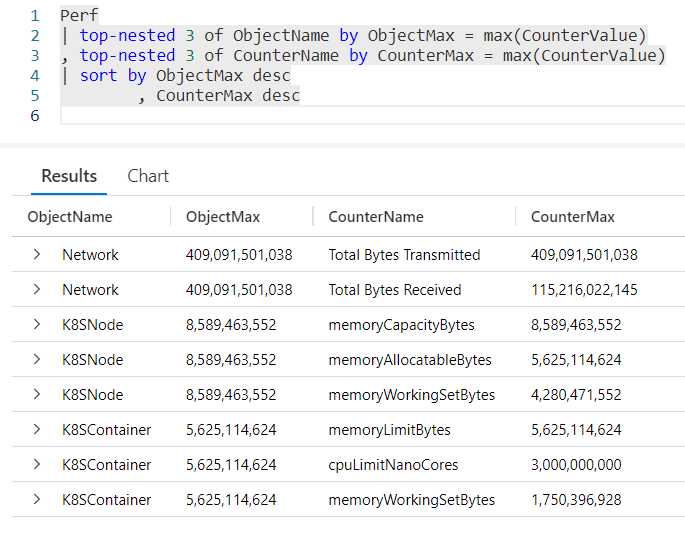
You can use max in many other places in KQL. As one example, refer back to my previous post Fun With KQL – Top-Nested. Instead of the count or sum aggregations we used in the post, we could have also used max.

In this example, we used the max function to rank our top nested values.

MaxIf

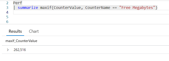
There is a variant to max called maxif. It allows us to include a condition in the second parameter such that in order for the value to be considered for max, the condition must be true.

In this example, we use CounterValue in the first parameter, then we put the condition CounterName == "Free Megabytes" in the second parameter, thus restricting the search for a maximum value to only rows with Free Megabytes in the CounterName.

As of now, you may not see much difference between using the combination of where and max versus the maxif. In a moment we’ll see another way to use maxif, but for now, lets move onto min.

Min

The min function can be used like max, except it returns the lowest value in the column indicated.

Here, we found the minimum CounterValue in the dataset that was passed in was 34.

Again, like max, the min aggregate function can be used in many places in KQL, like the Top-Nested operator.

MinIf

min also as an alternate version, minif. Just like maxif, you pass the column name as the first parameter and the condition in the second parameter.

Since it is so similar to maxif we’ll skip a detailed look at it for now, but we’ll show an example of it momentarily.

Max and Min as an Output Columns

It’s possible to include max and min as output columns in your query. In this example we used summarize to calculate the max and min values, giving them better names.

Using by CounterName will group the summarized values by their CounterName, and include the CounterName column in the output.

I used the in operator to limit to just two CounterNames, but you could include all of them, or your own set.

MaxIf and MinIf as Columns

In the previous example, we saw how to create columns to hold min and max values in the output. It had one drawback though. The values were for one of the two CounterNames we limited the results to. There was no way to distinguish which CounterName these values reflected.

This is where the maxif and minif aggregate functions come into play.

In this example we create four columns using the summarize operator. For each column we use either maxif or minif to create a value for just the CounterName we want.

maxif and minif can be used in other places as well. Think back to the previous example with top-nested. Perhaps we were only interested in a handful of ObjectNames.

The second line of the query could have been written:

| top-nested 3 of ObjectName
  by ObjectMax = maxif( CounterValue
                      , CounterName in ("CounterName1", "CounterName2")
                      )

This functionality would really let us hone in on just the data we need.

Conclusion

In this post we saw how to use the aggregate functions min and max. First we saw how to use them with summarize to return a specific value, then saw how to use them with part of another query. We also saw their alternates, maxif and minif.

The demos in this series of blog posts were inspired by my Pluralsight courses on the Kusto Query Language, part of their Kusto Learning Path.

Fun With KQL – Top-Nested

Introduction

Back in June of 2022 I covered the top operator in my Fun With KQL – Top post. We showed how to create your own top 10 lists, for example what were the top 5 computers ranked by free disk space.

What if you needed your top results in a nested hierarchy? For example, you wanted to know which three objects in the Perf table had the most entries? But, for each one of those, what were the three counters with the most entires?

That’s where the top-nested operator comes in. It allows you to create top lists in nested, also called hierarchical levels.

Before we begin our discussion on top-nested, you should be aware that the samples in this post will be run inside the LogAnalytics demo site found at https://aka.ms/LADemo. This demo site has been provided by Microsoft and can be used to learn the Kusto Query Language at no cost to you.

Top-Nested Basics

In the example below, we call the Perf table, and pipe it into our first top-nested operator. We then tell it how many items we want, in this case 3. Next, we tell it what we want three of, here we say we want the top 3 from our ObjectName column.

Next, after the by we indicate how we want to determine which ObjectName‘s are the top 3. Here we use the count aggregation, and storing that result in a new ObjectCount column.

OK, we’ve now setup the uppermost level for our top hierarchy. Now we need to tell the query what should be in the nested level. To do that, we use a comma, then a second top-nested operator.

Into the second top-nested we again say we want 3 items, this time from the CounterName column. Again we’ll rank these by the count aggregation, storing the result in the CounterNameCount column.

Finally we sort the results by the counts in descending order.

In the results, the first item was the Process object name, with 2,262,619 entries. It only had one CounterName associated with it, % Processor Time, which is why you only see one row for the Process object.

In second place is the ObjectName of LogicalDisk, with 1,286,540 entries. It had three counters associated with it. Of these, the Disk Read Bytes/sec took top place with 116,968 rows. In close second was Disk Bytes/sec with 116,965 entires in the Perf table. In third place for LogicalDisk was Disk Writes/sec.

The ObjectName that came in third was the K8SContainer, and you can see the three CounterName values associated with it.

Now that you’ve seen it in action, the top-nested operator is pretty simple to use and understand. Just tell it how many items you want, what item you want, and what aggregation you want to use to rank them.

Multiple Levels for Top-Nested

You can have many nested levels, in this next example we’ll use three levels of nesting.

Here we decided to get the top 5 of each level, and we went three levels deep, ObjectName, CounterName, then InstanceName. We could have gone even deeper, we just need additional top-nested operators for each level of our hierarchy.

Also note we decided to sort by the names of our various objects instead of the counter totals. This is a design decision that can be made by the ultimate end user of your query, and will be dependant on their needs.

Additionally, while I used 5 at every level, this isn’t a requirement. I could have used top-nested 3 at the ObjectName level, then top-nested 5 at the CounterName level, and perhaps top-nested 10 at the InstanceName level. Again, this can be determined by the needs of your end user, and Kusto is flexible enough to handle those needs.

Using Other Aggregations

So far we’ve been using the count aggregation for our needs. We can use any aggregation type we need to with top-nested. Take a look at this example.

Here, we used the sum aggregation, summing up our CounterValue column in order to determine the rank within our top-nested hierarchy.

We could have used other aggregations, such as min or max (both of which we’ll see in the next blog post), or any of the many aggregations available in Kusto.

All Others

Sometimes it’s just as important to know what wasn’t included in your top list. The top-nested operator gives us this capability through the with others capability.

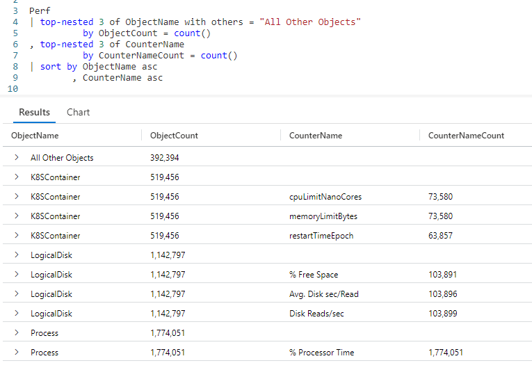
In this example, on the very top of the hierarchy you can see we’ve added with others = "All Other Objects" between the column to rank and the by. It is the with others that tells top-nested to aggregate the values not included in the final top list and display those results as well.

In the output, you see a row for "All Other Objects", this is the count for all the objects that were not in the top list.

The text All Other Objects was of my own choosing. I could have used any text here, like Not in the top list, Stuff not on top or Better luck next time.

Note that when determining the value for other it used the same aggregation function as the top-nested. Here we used count, but it could have been sum or whichever aggregation function we used.

Others at All Levels

In the previous example we only included others at the top level. We can use it at all levels if we wish. We’ll harken back to our original example with two top-nested levels, and include a others for each level.

In the second row, you can see K8SContainer, and All Other Counters in a sublevel, followed the the top 3 values for the CounterNames in the K8SContainer.

All Others at Sublevels Only

As you’ve seen many times in this Fun With KQL series, the Kusto Query Language is very flexible. This allows us a way to have others appear only at the sublevels, as you can see in this demonstration.

Here we only included with others at the second level of our nest. Do note this resulted in an extra row where the ObjectName is empty.

Conclusion

Getting a hierarchy of top items is a common business need. As you saw in this post, top-nested allows you to accomplish this easily. It also includes the ability to include the other values not included in the top-nested list.

The demos in this series of blog posts were inspired by my Pluralsight courses on the Kusto Query Language, part of their Kusto Learning Path.

Fun With KQL – Pivot

Introduction

Business Analysis is becoming mainstream in today’s corporate world. A big part of that analysis is done with pivot tables. Think of an Excel spreadsheet where data is organized into rows and columns.

The pivot plugin will take one data column from your query, and flip it to become new columns in the output data grid. The other column will become the rows, and an aggregation function will be at the cross section of the rows and columns, supplying the main data. You’ll get a better understanding through the demos in this post.

You may be wondering "plugin? What’s a plugin?"

Microsoft created a set of language extensions called plugins. These are functions which add extra capability to the Kusto Query Language. Plugins are invoked using the evaluate operator. pivot is one of the many plugins, we’ll look at more in upcoming posts.

Countries

Our ultimate endpoint for this demo is to get the count of requests, by the name of the request, for each country. In this demo we’ll be using AppRequests table, so lets begin by getting a list of countries.

For these demos we’ll start by using the AppRequests data, and filtering where the success was false, and the column containing the countries, ClientCountryOrRegion, is not empty.

To get our list of countries we’ll simply use distinct, then sort by the country column.

We’ll be using these countries as the columns in our output data grid.

Counts

Next, lets get the data that will be the basis for our pivot. We’ll project just two columns, Name and ClientCountryOrRegion. The Name column contains the type of request that was made, typically a GET or PUT request.

Now we call the summarize operator to get a count of the unique combination of Name and ClientCountryOrRegion and store it in RequestCount.

This does give us the data we need, the number of requests for each request type (the name) in each country. This data though, isn’t easy to read. For example, it’s difficult to compare the number of requests between countries.

We can solve this problem by using the hero of this blog post, the pivot plugin.

Pivot Basics

In this query, we get our data and project just the two columns we need. We then pipe this into the evaluate operator. As stated earlier, we have to use evaluate in order to call a plugin. Here, we follow the evaluate operator with the name of the plugin to call, in this case pivot.

Into the parameter of pivot we pass in the name of the data column from our query we want to become the column in the data grid. By default, the column not passed into pivot becomes the rows.

At the intersection of rows and columns is the aggregation function used by pivot. While there are several you can use (and we’ll see examples momentarily) by default if you don’t specify one count() is used.

After the call to evaluate pivot... we call sort, so the Name will be listed in ascending alphabetical order.

If we look at the first row, we see that "GET .aws/credentials" had one call, from the country of Russia. Looking further down, we can see "GET Employees/Create" had 1,355 calls, all in the United States.

Pivoting On A Different Column

The AppRequests table has a column ItemCount. What we want to accomplish with this next query is summing up the ItemCount value and have that be at the intersections of our pivoted table.

We need to make two modifications to the previous query. First, we have to add ItemCount to our list of projected values in order to use it in the pivot.

Next, we need to add a second parameter to the pivot plugin. We specify the type of aggregation we want to use, in this example sum. Then into the sum parameter we pass in the value to aggregate on, ItemCount.

In this case, at the intersection of the Name and ClientCountryOrRegion is the summed up ItemCount.

Other Aggregations

The pivot plugin supports many aggregations. The list includes min, max, take_any, sum, dcount, avg, stdev, variance, make_list, make_bag, make_set, and the default of count.

Be aware that these aggregations are used in many places in Kusto beyond just pivot. Over the course of these Fun With KQL blog posts we’ll be devoting posts to many of them.

Additional Columns In The Output

Sometimes you need more than just one column on the rows. The pivot plugin supports that in two ways. First, if you pipe multiple columns into it, all of them except for the pivot column you pass in are returned.

The second way is to pass the column names in as additional parameters, as you’ll see in this example.

Here, for the column to pivot on we once again used ClientCountryOrRegion, and our aggregation is sum of the ItemCount. Then we begin passing in the columns to display.

Be aware you need to pass in all the columns you want, if you omit any they won’t be in the results. In this example, we added Name and AppRoleInstance as the third and forth parameters to the pivot plugin.

I then used project-reorder, mostly for fun, you can read more about it in my Variants of Project blog post. Finally we call sort to sort the output.

While we could omit the columns as parameters and just use the default behavior of displaying everything passed in, explicitly listing the columns in the pivot parameters makes the query self documenting. It’s clear that we wanted these exact columns in the output. For that reason I prefer to list the columns as parameters.

Conclusion

In this post, we got introduced to plugins, and to the pivot plugin. We saw how to use it to create a pivot table for users to analyze data.

The demos in this series of blog posts were inspired by my Pluralsight courses on the Kusto Query Language, part of their Kusto Learning Path.

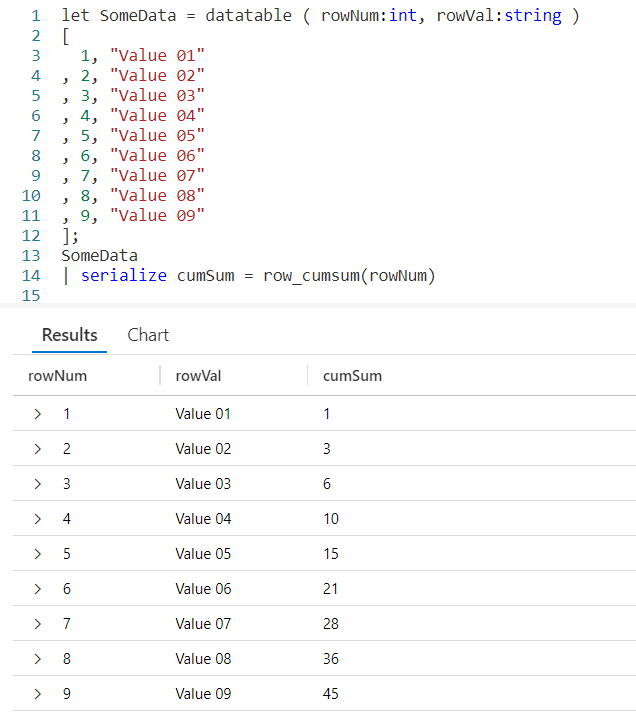
Fun With KQL – Contains and In

Introduction

Back on April 25, 2022 I did a blog post on the where operator, Fun With KQL – Where. In that post, I covered several functions that can be used with where to limit the results of a query. This list includes: startswith, endswith, has,hasprefix, hassuffix, and contains.

All of these had one thing in common, they were case insensitive. Kusto ignored the case of the text passed in. If you passed in the text BYTE, for example, Kusto would match on BYTE, Byte, bYtE, byte and other combinations.

There are versions of these which are case sensitive. We’ll see a few here, focusing on the contains keyword. In addition there are not versions, which will also be demonstrated.

There is another operator we’ll discuss here, in. It is a bit of an odd duck, in that it is case sensitive by default. We’ll see it and its variants later in this post.

Preface

For this section of the post I’m going to use contains for the demonstrations. Be aware everything I discuss on contains also applies to the other operators mentioned in the Introduction. Each has the same variants as contains.

Case Insensitive Contains

First, let’s take a look at the normal version of contains.

Briefly, we get the Perf table and grab three columns, TimeGenerated, CounterName, and CounterValue. This is then piped into a where, in which we use contains to look for rows in the CounterName column with the text BYTES.

In the results, you can see names like Available MBytes, Free Megabytes, and Bytes Sent/sec, to name a few. In this case the case of the text passed into contains, all uppercase, was irrelevant to the match.

Making Contains Case Sensitive

There is an alternate version of contains, contains_cs. Let’s rerun the above query, using the _cs version.

This invokes contains_cs, the case sensitive version of contains. It and will look for an exact match of the text that was passed in. In this case it looked in CounterName and found no records with BYTES in all caps, so in the results at the bottom shows "No results found…".

The other keywords I mentioned in the Introduction also have case sensitive versions, just add _cs to the end of their names.

Not Contains

In addition to the case sensitive versions of these commands, there is also a not version, as in "not contains". To invoke the not version of contains or any of the operators place a ! (exclamation mark, also called a "bang") on the front, as in !contains.

In the results you will see all rows as long as the word Bytes is not in the **CounterName column.

Note that the !contains is case insensitive. The casing of the value passed in, in this example Bytes didn’t matter.

Not Contains Case Sensitive

It probably won’t come as a surprise, but there is a case sensitive version of not contains. You simply combine the ! on the front and append the _cs to the end of the command. Here we do it with contains, using the command !contains_cs.

In this example we used !contains_cs to look for rows that did not contain the exact text BYTES in all caps. As you can see in the output, it returned rows including some that had the word Bytes, but it was in mixed case. No rows with upper case BYTES were returned.

In

In the introduction I mentioned there is one keyword that had the rules revered when it comes to case sensitivity, and that is in.

The in looks for values in a list that you pass into the in parameters. Let’s take a look.

We use where on the CounterName, then call in. In the parameters we pass in three values, three strings which we want to find rows with these values. The results show matches on some of the text that was passed in, there were many more rows not show on the screen capture.

One thing to note, by default in is case sensitive, unlike the other commands mentioned in this post. in looked for exact matches, including case, with the values we passed in.

Case Insensitive In

To make in case insensitive, you append a ~ (tilde) after the keyword, in~.

In this example, you can see it found matches for the values passed in, even though the case of the text passed in did not match the case in the results.

Not In

The in has a not version that works like the other operators. Place a ! (exclamation mark / bang) before it.

In this version of the query, !in returned all records except for ones in the list passed into the !in.

Also note we took advantage of the flexibility of the Kusto Query Language formatting and put each parameter on its own line.

Like a regular in, !in is case sensitive by default. There is a version, as you might expect, that can be case insensitive.

Not In Case Insensitive

To call the not and case insensitive version of in, simply combine the ! and ~: !in~.

With this example, it omitted matches of the three values passed in, regardless of the case of the text in the Perf table.

In Parameters

I just wanted to point out that with in there is no limit to the number of parameters. in can handle 1, 2, 3, 4, or more.

In addition, while these examples used strings in and its variants can also work with numeric values, for example where CounterValue !in (0, 42, 33, 73).

Conclusion

In this post, we covered how to make certain operators case sensitive as well as use the not versions of them. While we focused on contains, the same methods also apply to startswith, endswith, has,hasprefix, and hassuffix.

We then looked at the in operator and how it differed from the others when it comes to case sensitivity.

The demos in this series of blog posts were inspired by my Pluralsight courses on the Kusto Query Language, part of their Kusto Learning Path.

Fun With KQL – New Pluralsight Course! Kusto Query Language: Beginning Operators

Introduction

I’ve just published a new course at Puralsight, Kusto Query Language: Beginning Operators. This course is the second in Pluralsight’s Kusto Query Language Learning Path.

The Kusto Query Language can be used to retrieve and analyze data, not only in your own Azure Data Clusters, but for the health and status of your Azure-hosted infrastructure as well.

In this course, Kusto Query Language: Beginning Operators, you’ll learn the basic set of Kusto operators needed to author effective, useful queries.

First, you’ll learn to search across tables. Next, you’ll discover how to limit the data being output, as well as to limit the columns of data being returned.

Finally, you’ll explore how to add calculated columns to your query results. When you’re finished with this course, you’ll have the skills to write queries to answer a majority of your needs.

If you don’t have a Pluralsight subscription, there is a way to watch for free. Just go to my list of courses on Pluralsight . At the top is a Try For Free button you can use to get a free 10 day subscription to Pluralsight, with which you can watch my courses, or any other course on the site.

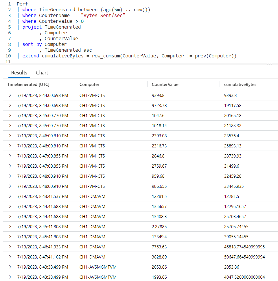
Kusto Query Language: Getting Started

If you missed it, I have a previous course in the learning path, Kusto Query Language: Getting Started.

The Kusto Query Language (KQL) is becoming increasingly important in the world of Azure.

In this course, Kusto Query Language: Getting Started, you’ll learn foundational knowledge of the Kusto Query Language.

First, you’ll learn what KQL is and where it is used, exploring the Log Analytics environment. Next, you’ll discover the basic structure, comparing it to other query languages.

Finally, you’ll explore the definitions of terms used with KQL. When you’re finished with this course, you’ll have the necessary skills and knowledge of the Kusto Query Language and the environments it is used in to begin authoring your own Kusto Queries.

You can also see this course for free, if you take advantage of the free trial described in the previous section.

Conclusion

As I write this, I have just completed recording the third course in the series, Kusto Query Language: Scalar Operators. It should be published around the end of January 2023.

I hope you enjoy the courses! And stay tuned to the blog, as I will be continuing my ongoing series Fun With KQL.

Fun With KQL – CountIf

Introduction

In my previous post, Fun With KQL – DCountIf, we saw how you could apply a filter to the data directly within the dcountif function.

You may have been thinking gosh, it sure would be nice if we could do that within the count function! (Note, you can read more about count in my Fun With KQL – Count blog post.)

Well fear not intrepid Kusto coder, there is just such a function to fit your needs: countif.

Count – A Refresher

Before we tackle countif, let’s refresh ourselves on how count works. Here’s a simple example.

We take our Perf table and pipe it into a where operator to only get back rows where our CounterName column has the word Bytes in it. Note for this example the contains doesn’t care about case, it’ll match Bytes, bytes, BYTES, and so on.

Next we flow into a summarize, which uses the count function to sum up by the CounterName column. Finally we do a sort to make the output easy to read.

CountIf Basics

Now let’s see how to do the same thing with the countif function.

First, we omitted the where since the filterning will be done in the countif.

Next we use summarize, and this time set a column name of RowCount to hold the value returned by countif.

In the countif function we pass a parameter, the expression we want to use for filtering. Here we use the same CounterName contains "Bytes" we used with the where statement in the previous example. We could have used any expression though; looked for an exact match using ==, used in with a list, or any other valid Kusto expression.

Finally, we used sort to sort the output.

Notice something different about these results as compared to the previous example. Here, countif included row counts with 0 values. In contrast, the count operator removes all rows with zeros before it returns the data.

No Zeros Here!

If we want the output of countif to match what count produces, all we need to do is add a where to suppress rows with zero values.

Here all we needed was to use where RowCount > 0 to remove those rows, making the output of countif match count.

No Guesswork Here

Just to be clear, countif, unlike dcountif, returns an exact value, not an estimate.

Conclusion

The countif function can provide a streamlined way to filter our data when we need accurate row counts. We just need to keep in mind it will return data with zero counts, which may be a benefit if your goal is to discover rows where the count is zero. Otherwise you just need to remember to filter those zero value rows out.

The demos in this series of blog posts were inspired by my Pluralsight courses Kusto Query Language (KQL) from Scratch and Introduction to the Azure Data Migration Service, two of the many courses I have on Pluralsight. All of my courses are linked on my About Me page.