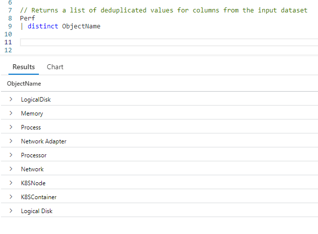
Fun With KQL – Parse_JSON and ToDynamic

Introduction

In order to compact data, JSON is often used to store information within columns in databases. JSON is also useful when you want to store data, but the exact data is different on a row by row basis. Using JSON prevents the need to have a lot of extra columns that will be blank for many of the rows.

It becomes important then that a query language provides a simple method for unpacking that JSON data into useful columns. The Kusto Query Language provides that ability through the use of the parse_json scalar function. In this post we’ll look at examples of how to use it to expand data stored in JSON format.

Originally, parse_json was called todynamic, and the older todynamic function name still works. Both functions work and behave identically. In this post we’ll use the newer parse_json name, but be aware that for any example you could use the older todynamic name and get identical results.

The parse_json samples in this post will be run inside the LogAnalytics demo site found at https://aka.ms/LADemo. This demo site has been provided by Microsoft and can be used to learn the Kusto Query Language at no cost to you.

If you’ve not read my introductory post in this series, I’d advise you to do so now. It describes the user interface in detail. You’ll find it at https://arcanecode.com/2022/04/11/fun-with-kql-the-kusto-query-language/.

Note that my output may not look exactly like yours when you run the sample queries for several reasons. First, Microsoft only keeps a few days of demo data, which are constantly updated, so the dates and sample data won’t match the screen shots.

Second, I’ll be using the column tool (discussed in the introductory post) to limit the output to just the columns needed to demonstrate the query. Finally, Microsoft may make changes to both the user interface and the data structures between the time I write this and when you read it.

Parse_JSON Basics

In order to use this function, we’ll need a table that has a column with JSON formatted data. For that we’ll be using the InsightMetrics table, which has a column named Tags.

Here is a sample piece of data stored in the column. Be aware that not every row in this table has the same format for its JSON data. In addition the samples in the code below may not match the screen shots exactly.

For this example I’ve broken the JSON code into multiple lines to make it easier to read. If you look at the JSON columns inside the results pane you’ll just see one long string of text.

 {
   "vm.azm.ms/mountId":"C:"
 , "vm.azm.ms/diskSizeMB":129545.99609375
 }

Now let’s see how to use parse_json in our Kusto query.

In order to properly use parse_json, each row in the dataset must have a consistent format for its JSON formatted column. So for this example we’ll take the InsightMetrics table, then use where to restrict the rows where the Name column is FreeSpaceMB. The Tags column for FreeSpaceMB rows have the required consistent JSON formatting.

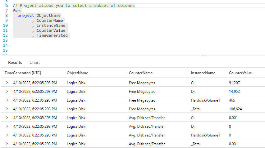
From here we use take to get a small sample for our demo (no sense in taking time to sift through 30,000 rows, the default maximum number of rows KQL will return in the user interface, for a simple demo). Next we flow into a project to just get the few columns we need.

Now we use the extend operator to create a new column, ExtProps. We use the parse_json function, and pass the Tags column into it. This will decompose the JSON data into the new ExtProps column.

In Kusto terms, they specify the new column as a datatype of dynamic. If you are familiar with PowerShell, this is actually created as a hash table, a list of key/value pairs. (If you aren’t familiar with PowerShell, you may want to take a look at my Fun With PowerShell) series.

Once we’ve unpacked the JSON into the ExtProps column, we flow into another project. The first three columns are a repeat of our original three.

Then we have our ExtProps column. In the first one, inside the square brackets [] we pass in the key we want, here vm.azm.ms/mountID. This will return the value associated with this key. If you refer to the JSON example above, this would be C:.

In the next ExtProps entry, we use the second key, vm.azm.ms/diskSizeMB. If you refer to the example above, this will return 129545.99609375.

In the image above, the last two columns are the unpacked JSON data.

More JSON columns

What if our JSON data was more than just two columns? Let’s take a look at an example with four key/values. As before I’ve expanded this to multiple lines to make it easier to read here, in the database it is all one long string.

{
  "container.azm.ms/clusterId":"/subscriptions/ebb79bc0-aa86-44a7-8111-cabbe0c43993/resourceGroups/CH1-GearamaRG/providers/Microsoft.ContainerService/managedClusters/CH1-GearamaAKS"
, "container.azm.ms/clusterName":"CH1-GearamaAKS"
, "hostName":"aks-nodepool1-18153691-vmss000000"
, "name":"sdb1"
}

We’ll again use the InsightMetrics table.

We use a where to limit the Namespace to container.azm.ms/diskio, the data associated with this Namespace has a JSON format that is consistent and resembles the four key/value pairs shown above.

We again use the same parse_json, passing in the Tags column.

In the project I simply reference the ExtProps column four times, passing in the keys for each one. I also used the project ability to rename these columns into something more human friendly.

Note, there is nothing special about the name ExtProps. I could have used any name I wanted, like TagProps, MyKeyValues, or even ArcaneCodeIsAwesome.

Case is Important!

Be aware, KQL is case sensitive when it comes to the JSON keys. When I was first developing these samples, I accidentally keyed in HostName = ExtProps["hostname"] then spent a few minutes scratching my head wondering why I wasn’t getting back any data for the HostName.

I finally realized I should have used hostName, and not hostname for the key (the N in Name is upper cased in the JSON). Once I got the casing correct, the query worked like it should have.

Property Notation

If, and only if, your JSON key has no spaces or special characters such as /, \, and so on, you can use what is called property notation.

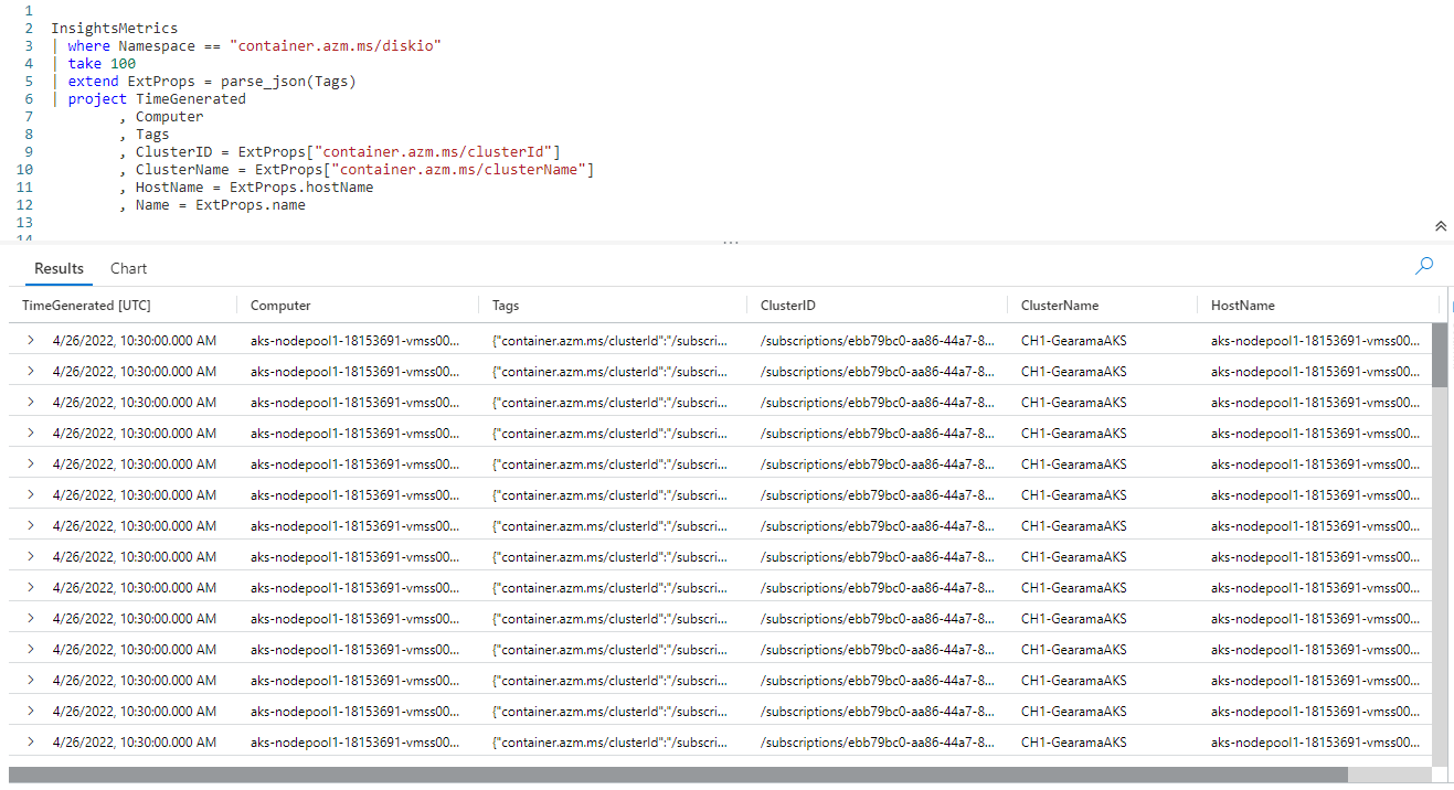
On the last two lines of the query, I was able to use ExtProps.hostName and ExtProps.name instead of needing to use the square brackets. This makes for a bit less typing and better readability. Note the case rules still apply with property notation, I needed to use hostName just as it was in the JSON.

For the ClusterID and ClusterName I still needed to pass the JSON keys within square brackets as they had special characters in the name.

Expanding Rows

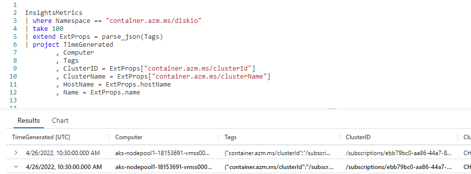
This is a good time to point out a feature of the user interface. In the results pane at the bottom, to the very left of each row you’ll see a sideways triangle. If you click it, it will expand the row to display the columns under it vertically.

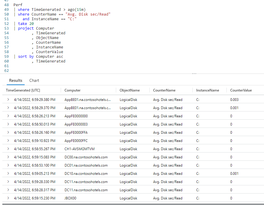
In this screen shot I clicked on the triangle on the second row (highlighted by the little red box in the image). This then expanded the row to display each column of data in a row under it. For results where many columns are returned, this can make it much easier to read the result for a specific row.

But wait, there’s more!

In the above screen shot, you may have noticed there is another arrow beside the Tags column. The interface figured out that the data contained in Tags is a dynamic datatype with JSON data.

Behind the scenes it used parse_json to unpack it, and break it into the individual columns (shown on rows under the Tags).

This is a useful tool for development. With this you can easily verify you are using the correct keys for writing your KQL code.

Conclusion

Finding JSON data stored in a database column is becoming more and more common today. It is fortunate that Kusto provides an easy to use way of extracting that data using the parse_json function. Remember for this to work in a query, each row must have a consistent format for its JSON.

I also want to add a final reminder, there is a version of parse_json named todynamic. Both functions work and behave identically, and can be used interchangeably. It’s important to remember this as you’ll find queries written both ways. When writing your queries though, you should prefer the use of the newer parse_json name.

The demos in this series of blog posts were inspired by my Pluralsight courses Kusto Query Language (KQL) from Scratch and Introduction to the Azure Data Migration Service, two of the many courses I have on Pluralsight. All of my courses are linked on my About Me page.

If you don’t have a Pluralsight subscription, just go to my list of courses on Pluralsight . At the top is a Try For Free button you can use to get a free 10 day subscription to Pluralsight, with which you can watch my courses, or any other course on the site.

Fun With KQL – Between

Introduction

It’s not uncommon to want to use a range of values when creating a Kusto query. This might be a range of numeric values, or perhaps a range of dates.

Kusto provides this ability using the between operator. In this post we’ll see how to use it when authoring your Kusto queries.

Just between you and me, the samples in this post will be run inside the LogAnalytics demo site found at https://aka.ms/LADemo. This demo site has been provided by Microsoft and can be used to learn the Kusto Query Language at no cost to you.

Between for Numeric Ranges

Let’s say you want to grab records from the Perf table for the percentage of free disk space. But you only want to see it when the CounterValue is greater than or equal to 70 percent, up to 100 percent.

You could write the where operator like where CounterValue >= 70 and CounterValue <= 100, but that gets a bit wordy. The between operator is not only easier to read, but is more efficient.

We start with the Perf table, then use a where to limit the dataset to only rows that hold the % Free Space counter data. We then use a take operator, to keep the demo sample small.

Now comes the star of this post, the between. Using a where, you specify the column name. Then comes the between operator. In parentheses, you place the starting value, two periods, then the ending value. Here, we go from 70.0 up to 100.0. This will include all rows with the starting value, 70.0, as well as rows with the ending value of 100.0.

In the results, you can see only rows in our specified range were included in the results. As I mentioned, the between is not only easier to read, it can be more efficient than using the where CounterValue >= 70 and CounterValue <= 100 construction I mentioned earlier.

Between for Date Ranges

In the introduction I mentioned you could use between for more than just a numeric range. It can also be used with dates.

In the where operator we used hard coded dates of April 12 to April 18, 2022. We had to put the dates in YYYY-MM-DD format. Because these are strings, we needed to use the datetime function to convert from a string to a datetime datatype.

In the result pane you can see all of our dates fell into the specified range.

Between Dynamic Dates

Hard coded dates may be OK for a quick, impromptu query, but for Kusto queries you’ll want to run repeatedly having dynamic dates makes more sense.

In this example we used ago(7d) to go back one week, with an ending date of right now by using the now function. If you want to read more about these two functions see the See Also section below for links to past articles I’ve written about them.

Not Between

Sometimes it makes more sense to write your Kusto query to exclude a range. For that, KQL includes a not between operator.

In this example we used !between to exclude counter values in the range of 0.00 up to and including 69.999. This produced the same results as our first example.

Conclusion

Using the between operator allows you to not only write more readable queries, but ones that are more efficent.

Fun With KQL – EndOf

Introduction

My post, Fun With KQL – DateTime Arithmetic, demonstrated how to do date / time math in Kusto. Then in my previous post, Fun With KQL – StartOf, we showed how to use the StartOf... functions, to calculate the beginning of time periods based on a date that is passed in.

If you’ve not read the previous post I’d highly encourage you to do so now, as there are parallels between it and the endof... functions we’ll discuss in this article, namely endofday, endofmonth, endofyear, and endofweek.

The samples in this post will be run inside the LogAnalytics demo site found at https://aka.ms/LADemo. This demo site has been provided by Microsoft and can be used to learn the Kusto Query Language at no cost to you.

EndOf Basics

Let’s start with a simple query. We’ll take the TimeGenerated column from our query and add a new column to display the end of that day.

We took our Perf table and piped it into the where operator to get all rows since the start of the current year. That in turn was piped into a take, to grab just a few rows for this demo.

Now our function comes into play. We use the extend operator to create a new column, DayGenerated. This is set equal to the endofday function, into which we pass the TimeGenerated column.

Finally we use a project to limit the columns to the results pane a the bottom.

In the results pane you can see the two date columns, TimeGenerated and DayGenerated. The both show the same date, but the time in the DayGenerated column will always be 11:59:59.999 PM. This time is always returned for an endof... functions return value, whether you use endofday, endofmonth, endofyear, or endofweek.

Summarize by End of Day

Let’s turn to common use for the endof functions, the ability to summarize for a time period.

As in the previous example we piped Perf into a where to limit to data from the start of the year. Then we used extend to add a new column which is the end of the day for the TimeGenerated column.

We then used project to narrow down the list of columns. From here we used the summarize operator to create a count of the number of entires into the Perf table based on the new DayGenerated column and the name of the Computer.

Summarize by End of Month

We can also create summaries for the end of each month.

This query is the same as the one in the previous end of day section, except we use the endofmonth function. In the output you can see, for the computer AppBE00.na.constosohotels.com, we get the last day of each month from January 2022 until April 2022. Note it is April 2022 as I write this, so April is the most recent month we have data for.

Summarize by End Of Year

I’m sure you are getting the hang of this by now, even so let’s see a few more examples. Here, we’ll summarize by the end of the year.

In the where clause of this query, I used startofyear( now(-768d) ). I showed this technique in the previous post Fun With KQL – StartOf. Passing in a negative value into the now function subtracts that many days from the current date.

As there are 365 days in a year, we double that to get 768. It’s April 21, 2022 as I write this, thus it would return April 21,2020. The start of that year was January 1, 2020. Thus the where clause will return all rows where the TimeGenerated is greater than January 1, 2020.

In this case it doesn’t make a great deal of difference, since the sample data doesn’t go back that far, but I wanted to take this chance to remind you of the techniques to return several years worth of data in your query, especially as doing year end summaries would often be done jointly with returning multiple years of data.

Summarize by End Of Week

As our last example, lets see the endofweek function used alongside the summarize operator.

This query works as the others, except of course we use the endofweek function. In the results pane you can see the WeekGenerated column has the last day of each week, by default a Saturday. This is in contrast to the startofweek function, where weeks start on Sundays.

Conclusion

In this post we saw how to use the endof... series of functions to calculate period ending dates dynamically. We then saw how to use the various endof... functions to group data into discrete time buckets using summarize.

Fun With KQL – StartOf

Introduction

In the previous post, Fun With KQL – DateTime Arithmetic, we had hard coded a date for the start of the year, in order to find out how much time had elapsed between it and datetime columns. I had mentioned there are ways to dynamically calculate such values.

In this post we’ll look at one way, using the StartOf... functions. These include startofyear, startofday, startofmonth, and startofweek.

Before we get into the StartOf... collection of functions, I want to point out that the samples in this post will be run inside the LogAnalytics demo site found at https://aka.ms/LADemo. This demo site has been provided by Microsoft and can be used to learn the Kusto Query Language at no cost to you.

StartOf Basics

In this first example, we’ll use two of the StartOf functions.

First we use the startofyear function in the where operator to return all rows whose TimeGenerated occurred since the start of the current year. That would be 2022 as I write this, but would calculate back to January 1 for whatever the current year is.

Next, as I’ve done in past articles I use the take operator to keep our sample small, since this is just a demo.

The next line uses the extend operator to add a new column, DayGenerated. It uses the startofday function, into which we pass the datetime column of TimeGenerated.

The start of the day will always begin at midnight, 12:00:00.000 AM.

From here we flow into a project to display the essential columns. In here you can contrast the TimeGenerated column with our new calculated column of DayGenerated.

StartOf Previous Years

In the previous example we returned the start of the current year. What if we wanted the start of last year? Well that is pretty easy with a little math.

In this example, we simply took now and passed in an off set of -365d, or 365 days in the past, putting into last year.

It’s April 20, 2022 as I write this, so that would return April 20, 2021. Using that date, startofyear willl return January 1, 2021.

Need to go two years back? No problem, just multiple the offset of -365 by the number of years.

Two years ago would be 365 * 2, or 768 days in the past. Sure enough we get a date of January 1, 2020.

Summarize by StartOfDay

Let’s move on to do something more useful. In previous articles we’ve used the summarize operator to summarize counts by things like the computer name, or perhaps the counter name.

We can use the startofday function to return the number of entries into the Perf table for each day.

As before, we pipe Perf into a where to get results since the start of the current year.

Next, we use an extend to calculate the DayGenerated, using the startofday for the TimeGenerated.

We then project only the few columns we need. The summarize operator comes next, so we can get counts for each Computer for the day the data was generated. Finally we sort by the computer name and day generated in the output.

The result is a common use for the startofday function, one you will probably use frequently.

Summarize by StartOfMonth

Getting monthly summaries of counts is also a common need, so let’s employ the startofmonth to get these.

As you can see, our query is identical to the previous one, except of course for the use of the startofmonth function. In the output, you can now see the log counts for each month, broken out by computer name.

Summarizing By StartOfYear

Once again, we can use another startof function to summarize by year.

Again, just like the previous query except we use startofyear in the summarize operator. Note too we could have used now(-365d) to get this year and last years data, although in the sample database most of the tables only have current year data.

Summarize by StartOfWeek

One last example, we can do summaries by week.

Here you can see using startofweek in our query resulted in weekly buckets for our data. This can be helpful when we want to compare data week over week. By defaults weeks start on Sunday.

Conclusion

In this article we used the startof... collection of functions to limit the data being returned as part of our where operator. We also saw how these functions could be used to group the data into discrete buckets of time.

Just like startof..., there are a corresponding collection of endof... functions, which we’ll examine in the next article.

Fun With KQL – DateTime Arithmetic

Introduction

Performing DateTime arithmetic in Kusto is very easy. You simply take one DateTime data type object and apply standard math to it, such as addition, subtraction, and more. In this post we’ll see some examples of the most common DateTime arithmetic done when authoring KQL.

DateTime Arithmetic Basics

In our first example we’ll do something extremely common. We want to know how long ago something happened.

We start by grabbing the Perf demo table, then piping it through two where operators to limit the data. That is piped into a take operator to give us a small sample set. Since this is just a demo we didn’t need 30,000 rows.

Now we fall into an extend, which is where the fun happens. To see how long ago this row was logged into the Perf table, we simply subtract the TimeGenerated column from the now function, which returns the current datetime. I then assigned this calculated value to the column name of HowLongAgo, to prevent KQL from assigning it a dumb column name like Column1.

I wrapped the calculation in parenthesis. Technically this wasn’t required, it was just to demonstrate the flexibility of the Kusto query language. Sometimes using an item like parenthesis, even when not needed, may make your code more readable.

Within the extend I added a second column RightNow and set it equal to now. This was just so you could see the value being used in the previous calculation.

Finally I pipe to a project to grab the few columns we need to verify our output.

Time Since A Date

Another use for DateTime arithmetic is determining how long it has been since a specific date. In this example we’ll determine how long it has been since the start of the year 2022 (the current year as I write this).

The only difference with this query and the previous one is the addition of a new calculated column, TimeSinceStartOfYear. In it, we want to subtract the start of the year, January first, from the TimeGenerated.

In order for date arithmetic to work, all components must be of a datetime datatype. We know the TimeGenerated column is already a datetime, so we’re good to go there.

In order to convert a hard coded date, in this case January first of 2022, we need to use the datetime function. This will take the string passed in and make it a datetime datatype. The format passed into datetime needs to be in YYYY-MM-DD format.

In the results pane, you can see the first row shows 103 days, 18 hours, 33 minutes, and 26.037 seconds since the start of the year!

In this example we hard coded the date, in later posts we’ll show how to calcualte things like the start of the current year using functions built into Kusto.

Note, the resulting column from this calculation, TimeSinceStartOfYear, is not a datetime datatype, but rather a datatype of timespan.

Timespan Results In Specific Units

In the previous example, we calculated the time since the start of the year until an event was logged in our Perf table. It returned the value in a timespan which had days, hours, minutes, and seconds.

What if we needed the time returned in a single unit such as hours? Well that is possible too, using just a bit more date arithmetic.

With the first extend operator, we created a new column, TimeSinceStartOfYear, which resulted in a timespan datatype. Now we want to express that new timespan in hours.

We can take our new column and pipe it into a second extend. In here we’ll divide the timespan by the unit we want, in this case hours. In the output this resulted in 2,490,557 hours since the start of 2022.

Any unit could have worked, 1d would work for days, and is very common for larger timespans. Seconds (1s) and minutes (1m) are also useful.

You’re not restricted to single units either. You could, for example, have used 7d to return how many weeks are in the timespan, or maybe 365d to see how many years.

One note, you’ll see a lot of repeating values in the output. This is strictly due to this being sample data from Microsoft.

Date Arithmetic Between Columns

So far all of our calculations have been between a date and a function, such as now, or a fixed date (cast using datetime).

We can also perform datetime arithmetic between two columns in a dataset.

In this example we’ll use a different table in the Log Analytics database, Alert. When a query is executed it places that event in the Alert table. Included are two columns, which indicate when the query started and when it ended.

We’d like to know just how long each query took to execute. In this example we took the Alert table and piped it into a take operator to give us a small sample set for this demo.

From there we pipe it into an extend where we do our date arithmetic. All we have to do is subtract the QueryExecutionStartTime from the QueryExecutionEndTime to give the timespan the query took. Yes, it is just that easy, and results in a timespan.

We then pipe that into a project operator and display the results. As you can see, the QueryExecutionTime calculated column resulted in ten minute query times.

Again, like most of the examples in this Fun With KQL series, there are a lot of duplicated values due to this being sample data.

Conclusion

In this post we covered the basics of datetime arithmetic. There are more functions that can be used with datetime arithmetic, which we’ll see in upcoming posts in this series.

Fun With KQL – Parse

Introduction

The previous post in this series Fun With KQL – Extract, showed how we can use the extract operator to pull part of a string using regular expressions. I think you’d agree though, using regular expressions can be a bit tricky.

If you have a string that is well formatted with recurring text you can count on, and want to pull one or more strings from it into their own columns, Kusto provides a much easier to use operator: parse.

Before we get into parse, be aware that the samples in this post will be run inside the LogAnalytics demo site found at https://aka.ms/LADemo. This demo site has been provided by Microsoft and can be used to learn the Kusto Query Language at no cost to you.

Parse Basics

The AppRequests table in the LogManagement section of the Demo database has a column called Name. The Name column always begins with the word GET followed by a space, then the request that was passed in.

What we’d like to do is return just the data that was being requested by the GET.

In this example we take our AppRequests table and pipe it into a take operator to keep our sample set small.

Now comes the parse. After the operator we give the name of the column we want to parse, in this case Name.

After the with comes the string we want to look for, here it is our GET . (Make sure we include the trailing space after GET.) Kusto will look for the string, then start grabbing the characters after it.

It will keep grabbing characters until it either hits the end of the string, or until it finds a match for a second string we pass in. We didn’t pass in a second string with this example (that will come in the next section), so it just keeps going until it hits the end.

That data is then placed in the new column name we provide, here I used ParsedGet although we could have used any name.

If you look at the output, we have the original Name column, then we have the new ParsedGet column. As you can see, the GET is now missing from the ParsedGet column.

Parsing Multiple Columns

That was easy! What if we wanted to extract multiple parts from a string?

Let’s take a look at the table FunctionAppLogs. It has a column, Message. When the category is Function.Function2 and the level is Error, the Message column will always have the message formatted the same way.

It will begin with the text Executed 'Function2' (Failed, Id=. After this is the ID of the error.

After the ID comes the text , Duration=, then the duration of the error in milliseconds. The final bit of text is a right parenthesis. Lets see how to extract this text so we can get the ID and the Duration as separate columns.

Here we have the parse operator, then the name of the column to parse, Message, then the with keyword.

We then enter the text we want to start looking for, Executed 'Function2' (Failed, Id=. The parse operator will start getting characters right after the equal sign.

It keeps going until it finds the text , Duration=. At that point it stops, and copies the characters it has found so far into the new column, which we named FailedID.

Once it has done this, it begins to look for more characters after , Duration=. It keeps taking those characters until it finds the third string, ). That data is then placed into our column which we named Duration.

The parse operator then finds the ), and starts looking for more characters until it gets to the end of the text, and would put that into a column we named NoOutputHere.

Because parse didn’t find any characters after the ), nothing is placed into NoOutputHere. At the end of our query, since the NoOutputHere column is empty for all of the rows, it is discarded from the final output.

This little trick can be a handy way of removing any unwanted characters from the end of a text string, in this case the closing parenthesis.

Also note that unlike other operators in Kusto we do NOT separate the passed data with commas.

Looking at the output, you can see the FailedID column now contains only the ID part of the Message column. Likewise, the Duration column contains only the duration piece of the Message column. As I just mentioned, Kusto helpfully discarded the closing parenthesis from the output.

In this case we only extracted two pieces of data from our string, but we could have kept going adding more text to look for as part of our with statement.

When You Can Use Parse… and When You Can’t

Parse works great when the format of the text string is always the same, as was the case in this example. If not, you will need to find ways to narrow down the dataset until it is.

Let’s see this quick example…

If you look closely at the Message column, you’ll see the message text differs between levels Error and Information. As such our parse from the previous section would not work. That’s why we had to add the and Level == "Error" in the previous query, to limit the rows so our Messsage column had the same text format for every row.

Conclusion

The parse operator can be extremely useful for extracting portions of a string, and breaking them out into columns, without the need for complex regular expressions. As long as, that is, your columns text has a consistent format.

Fun With KQL – Extract

Introduction

Almost all languages have the ability to extract part of a string. In C#, this is the Substring method of a string. With SQL, it is the SUBSTRING command.

Kusto has an operator that will perform this same task, it is called extract. In this post we’ll see some examples of using it.

Extract Basics

In this example, we want to extract the drive letter information from the InstanceName column.

We start with a standard query, taking the Perf table and piping it through a where operator to limit the dataset to ObjectName of LogicalDisk and using a regular expression to only get instances of drive letters.

Next we use a take to grab 20 random rows, to keep the sample data for this post small. This is then piped to a project to select just a few columns.

In the last column we employ the extract function. The first parameter is a regular expression that will grab a single letter in the range of A to Z, followed by a colon.

The second parameter, 0, indicates we should grab the entire text returned by the regular expression. In the output this is C:, D:, and so on.

The third and final parameter passed into extract is the column name we want to extract from, InstanceName. Finally we assign the result to the column name of DriveLetter, a name we picked. We could have called it Fred if we wanted, or omitted it entirely.

Extracting Part of a String

We also have the option of returning part of the text.

In this example, we wrap the [A-Z] in parenthesis. We then pass a 1 as the second parameter to the extract function. This tells extract to only return the portion of the string within the parenthesis.

In the output, you can see the DriveLetterOnly column only has the single drive letter, it omits the column.

Extracting Multiple Characters

In addition to a single character, the extract can grab multiple characters. You need some good regular expression skills to do so.

In this example we are using the distinct operator to get a unique list of computer names from the Perf table. We grab 20 random rows to keep the sample small, then go into a project.

In the first parameter to extract, inside the parenthesis, we pass in [A-Z]{2,4}. This translates to "look for upper case characters in the range A to Z, where there are between 2 and 4 of them in a row".

As before, the 1 parameter only returns the data in the parenthesis, and the third parameter is the column we want to look in.

In the output you see a list of matches in the PartialText column. When the PartialText column is blank, it means it did not find a match.

As you can see, you’ll need good skills at regular expressions to formulate good matches, but it can be done.

Conclusion

Extracting parts of a string is a common need when authoring queries. In this article you saw how to use the extract function, combined with regular expressions, to accomplish this.

Fun With KQL – Sort

Introduction

Like most query languages, the Kusto Query Language as the ability to sort the output. It works almost, but not quite, like you expect. So let’s take a look at the KQL sort operator.

First though, let me mention the samples in this post will be run inside the LogAnalytics demo site found at https://aka.ms/LADemo. This demo site has been provided by Microsoft and can be used to learn the Kusto Query Language at no cost to you.

Sort Basics

Using sort is just about like you’d expect. You take your query, and pipe the output into the sort operator. After the by you simply list the column or columns to sort by.

Here we pipe our Perf table into two where clauses to first reduce the output to the last 15 minutes using ago, then further reduce for only rows with a CounterName of Avg. Disk sec/Read and the InstanceName of C:.

From here we use a take, to grab 20 random rows just to keep this result set small for the demo. A project follows, to reduce the columns we want.

Finally is our sort operator. It will sort our output first by the Computer column, then by the TimeGenerated. (If you need further info on any of these commands, refer to the See Also section below.)

Now take a look at the output, specifically the Computer column. You’ll see we have computers with SQL first. Then there’s a Retail computer, then some entries for JBOX.

"Wait!" you might be yelling at your computer. "That’s not sorted right!"

Well in fact it is, since by default the sort operator sorts in descending order. With text based fields, like Computer, it sorts Z to A.

With numeric fields it sorts biggest to smallest, and with dates the most recent to the farthest back in time.

Frequently you want to get the biggest values for troubleshooting. Which computers had the biggest network latency? Which computers have the largest amount of disk space used? Hence the developers of Kusto chose to have the default for sort be descending.

Sort in Ascending Order

Not to worry though, it is easy to get your output to sort in ascending order.

All you have to do is place the asc keyword after the column name, and it will now sort smallest to largest. As you can see, the Computer column now starts with the A’s, then C’s, and so on. Likewise the TimeGenerated starts with the oldest, then works its way forward in time.

Mixed Sorting

The nice thing about placing the sort order after the column name is that you can set the sort order for each column independent of the other columns.

Here we simply removed the asc after the TimeGenerated column in the by. Now the Computer column will sort alphabetically, A to Z, but the TimeGenerated will sort in descending order, most recent to oldest.

There is actually a desc keyword you can use.

In terms of syntax, it makes no difference whether you use desc or not, as descending order is the default. However, I personally think it makes a big difference in terms of readability.

If you have asc on some columns, but not others, readers of your query (including you later) may wonder "well did they intend to sort in descending order, or did they forget to put an asc on the end?"

By explicitly having the desc in the query, you remove all doubt. Yes indeed, you meant for this column to be in descending order. As such I’d encourage you to always use desc whenever you have asc as part of your sort operator.

Order By

Are you coming to KQL from an SQL world? Well to make it easier, Kusto includes an order by operator.

The order by is just a synonym for sort by. As such it behaves exactly the same.

Conclusion

In this post we saw how to sort your query results using the sort operator. We learned that it defaults to descending order, but you can override that with the asc keyword. Finally we learned about the synonym for sort by, order by.

Fun With KQL – Ago

Introduction

The ago function is very similar to the now function, which was discussed in my previous post Fun With KQL – Now. In this article we’ll take a look at ago, see how it works and how it differs from now.

We’ll be using both the print operator and the now function in this post, so if you aren’t familiar with them please go read my articles Fun With KQL – Print and Fun With KQL – Now.

In addition, I also use the where operator, documented in Fun With KQL – Where, the extend operator, which I discussed in the article Fun With KQL – Extend, and take, which you’ll find more information in Fun With KQL – Take.

Ago Basics

The ago function allows you to pass in a time offset in as a parameter. It will then go that length of time into the past and retrieve the date. For example, to get yesterdays date, we would pass in a value of 1d.

Below is a chart of the time span notations you can use.

Abbreviation	Time Unit
d	days
h	hours
m	minutes
s	seconds
ms	milliseconds
microsecond	microseconds

As you can see in the output, ago, like the now function, works with a variety of time spans. For this example we used the simple 1d, but the number can be anything. 365d, 12h, 30m are all valid time spans to use with both ago and now.

Ago vs Now

The big difference between ago and now is the way they handle input parameters. When you pass in a positive value into ago, it goes that many time spans into the past. With now, it goes that many time spans into the future.

The current date (when I did the screen capture) is April 13, 2022. Passing in 1d to now returned April 14th, where the same 1d into ago returned April 12.

So what happens if we pass in negative values to these functions? As it turns out, ago winds up behaving like now, and now behaves like ago.

With now being April 13, passing in a negative -2d to now gives us a date two days in the past, April 11.

Likewise, passing in a -2d into ago, gives us two days in the future.

Using Ago In Queries

The most common use of ago is in queries, combined with the where operator, to limit results for the last hour, day, or other time span.

Here, I used the where operator, combined with the ago function, to say "give all rows that occurred within the last hour".

I then added an extend operator to add the current date time (using now) just to show the current time. This isn’t something you’d normally do, but I wanted it to illustrate this concept. Finally it is piped into the take operator to give just a few rows for this sample.

In the output, the RightNow showed the current time when I ran the query was 9:45 pm. Thus, one hour ago would be 8:45 pm. As you can see in the TimeGenerated column, all of the times were after 8:45 pm.

Why Have Ago AND Now?

So after learning about these two functions, which essentially do the same thing, you may wonder "why have both ago and now?"

Simply put, readability. When we see negative values, the brain has to stop and think a moment about what is going on. Having both functions avoids this.

When you see ago, your brain automatically understands this is generating a date in the past. When you see just now(), you instinctively know this is the current date. Finally, if you see now with a parameter you know this is calculating a date in the future.

By the way, you can also make ago simulate now by passing in a time span with a value of 0 (zero).

Here I used a d for the time span, but any time span notation would have worked, 0m, 0s, and so on. I don’t actually recommend this however, this is a case where you really should be using now. I just wanted to mention it in case you happen to encounter it at some point in the future.

Conclusion

In article we covered the use of the ago function to calculate dates in the past. We contrasted it with the now function, and learned when to use each of these functions to make our code more readable.

Fun With KQL – Now

Introduction

What time is it? That’s what the KQL function now will tell you. It will return the current date and time. It is mostly used in queries where you need data relative to the current date and time.

Before we go on, let me mention the samples in this post will be run inside the LogAnalytics demo site found at https://aka.ms/LADemo. This demo site has been provided by Microsoft and can be used to learn the Kusto Query Language at no cost to you.

Now Basics

At its simplest, the now function returns the current date and time.

Here we used the print operator (covered in Fun With KQL – Print) to display the current date time to the results pane at the bottom. Just a reminder, all Kusto functions require the use of parenthesis at the end, even if they are left empty.

Now With An Offset

The now function can accept parameters. You can enter an offset to return a date in the past, or future, relative to the current date and time.

In the first column I get the current date time with now() and copy it into the RightNow column of the output.

In the second column I pass in a parameter of -2d to now. This will subtract two days from the current date time and place it in the TwoDaysAgo column.

Finally, I pass in a value of 4h to now. This will get the time four hours in the future, again from the current date and time.

Below is a quick reference for common date and time abbreviations that can be passed into Kusto’s many date time functions, including now.

Abbreviation	Time Unit
d	days
h	hours
m	minutes
s	seconds
ms	milliseconds
microsecond	microseconds

Using Now in a Query

You can also use now as part of a query, as well as in its calculations.

Here, we took the Perf table and piped it through two where operators to limit the dataset to only rows with a counter name of Free Megabytes whose counter value is greater than zero.

It is then piped through the take operator to give us a small sample dataset of ten rows to work with, for demonstration purposes.

Next we use the extend operator to add a new column to the dataset naming it HowLongAgo. To get this, we subtract the TimeGenerated column from now(), to see how far in the past this entry was recorded in the Perf table. If you look at the value in the first row, the HowLongAgo indicates this data was recorded 0 hours, 20 minutes, and 20.9790581 seconds previous to the current date time.

The project operator is then used to get only the columns we want, including making a copy of the current date time (using now) into the CurrentTime column.

If you’re not familiar with the operators that were used in this query, you can refer to my past posts for more information.

Fun With KQL – Where

Fun With KQL – Take

Fun With KQL – Extend

Fun With KQL – Project

Conclusion

In this post we covered the useful now function. It is a function you’ll use a lot in your work with Kusto. In the next post we’ll look at the other common date function ago, and contrast it with now.

Fun With KQL – Print

Introduction

In this post we’ll cover the print operator. This Kusto operator is primarly used as a development tool, to test calculations.

Print Basics

The print operator is very simple. It simply takes the expression after the print operator and returns it to the results pane at the bottom.

We passed in a static string of "Hello World" and it was displayed at the bottom.

A bit more useful job for print is to verify the formatting of a calculated string using strcat. Perhaps it is one that involved multiple column names. You could create and test a rough draft using print.

For this example, I want to take four columns and create an output that reads like a normal sentence. Getting the formatting just right can often be a bit of trial and error. Even more, you don’t want to keep running long queries just to test your output string formatting.

This is where the print operator comes in handy. Here you can see I used placeholders for the column names, surrounding them in double asterisks (although that’s not necessary), then included the static strings I’d be using in the final query. This lets me verify I have the spacing right, decide if I like the look of the output, and so forth.

Print and Calculations

More commonly, you might use print to verify a calculation.

Normally your calculations would be more complex, but it would give a way to enter and test it before you apply it to a column of data in a later query.

If you want, you can even give your calculated column a name.

Simply assign a column name prior to the calculation. In the output grid at the bottom you can see it now used the name for the column.

Print and Dates

A frequent use for print is to verify dates. In an upcoming post I’ll cover the ago function in depth, but briefly you can pass in a value to see what the date would be a certain number of days in the past.

Perhaps you have a query that relies on using ago to get the date for one year ago, but it doesn’t seem to be working right. You can use print to see what date Kusto is calculating.

This lets you verify if the date you think is being used is, in fact, the date Kusto is using.

Conclusion

In this post we covered the use of the simple print operator and some of its uses. Hopefully you’ll find creative ways to use it as you develop your Kusto queries.

Fun With KQL – Top

Introduction

Top 10 lists are all the rage on the internet. Everywhere you look you see "Top 10 Cute Kitten Videos" or "Top 10 Pluralsight Videos by ArcaneCode".

KQL includes a top operator so you can generate your own top lists. Even better, you are not limited to just ten items either.

Top Basics

Using top is straightforward. Simply pipe a dataset into the top operator, indicate how many items you want, then what you want to use to measure the top with.

By using top with the TimeGenerated datetime column, and adding desc to get descending order, we get the most recent 20 rows that are in the Perf table.

Top Troubleshooting

The top operator has many potential uses. In a financial system it could be used to retrieve the top 10 transactions by monetary amount. Beyond such obvious uses, top can also be useful as a troubleshooting tool.

For example, lets say we want to get a list of computers with low disk space as recorded in the Perf table.

Since we don’t want to look at every single row, as the same value may have many entires, lets reduce the dataset by using the distinct operator to just the computer, counter name, and counter value.

Finally, we use top to get the top results sorted in ascending order (least free space to largest) by the CounterValue, which in this case is the amount of free disk space in megabytes.

Now we have a list of computers reporting a low disk space. In this case they all have 34 megabytes free, but that is due to this being a sample database.

Conclusion

In today’s post, we covered the top operator, and saw several ways it could be used. Hopefully you’ll be able to use this operator to get your queries in "top" shape!

Fun With KQL – Distinct

Introduction

As with other languages such as SQL, KQL has an operator for returning a unique list of values in a column: distinct. Using this you can return the values in a column, but only once, removing any duplicate values from the result set.

Distinct Basics

Using distinct we can get a list of unique values in a column. Let’s say we want to get a list of distinct values in the Perf tables ObjectName column.

All we had to do was take our Perf table and pipe it into the distinct operator. We then specify the column name to get the unique values for.

In the output, you can see the list of values. You could use these to build a lookup table, or as input to another query.

Distinct Combinations of Columns

When using the distinct operator you are not limited to a single column. You can get distinct values for a combination of columns.

After distinct we simply list all of the columns to find unique combinations for. In this example, you can see the LogicalDisk object has several counter names associated with it. It was too long for a screen capture, but in total the query returned 43 unique combinations. (As of this writing, be aware the value may be different for you due to the constant updates to the Perf tables sample data.)

Distinct As A Troubleshooting Tool

One way you can use distinct is as a trouble shooting tool. There is another table in the LogManagement solution named Alert. In here certain conditions which may become issues are logged. You can use the distinct operator to get a list of those conditions.

When I ran this query, it only returned one alert condition, but there could be more. We can now use this information to get a list of the computers that raised this specific issue.

With the list of computers narrowed down, we can start investigating each one to see what raised this issue.

Conclusion

It was my "distinct" pleasure to bring you this article on distinct!

OK, sorry for the bad pun, but hopefully you learned some ways the distinct operator can help you in your work.

Fun With KQL – Variants Of Project

Introduction

In the previous post, Fun With KQL – Project, we took a dive into the project operator and the ways it could be used. The project operator has several variants: project-away, project-rename, project-keep, and project-reorder. This post will take a quick look at each.

For most of the examples we’ll build on the examples from the Fun With KQL – Project blog article, so if you’ve not read it you should do so now.

You should be aware that the samples in this post will be run inside the LogAnalytics demo site found at https://aka.ms/LADemo. This demo site has been provided by Microsoft and can be used to learn the Kusto Query Language at no cost to you.

Project-Away

There are several variants to the project operator. The first I wanted to mention is project-away.

The project-away operator is the reverse of project. It will return all columns except the ones you indicate. This can be a way of future proofing your queries. With project, if someone adds a new column to the table it won’t appear in the results. With project-away, these new columns will now appear in the results.

To be honest, the project-away operator isn’t something I’ve used a great deal, but wanted to include it for completeness.

Project-Rename

Another variant to the project operator is project-rename. You can use it to rename a column. As this example shows, that renamed column can also be used in calculations done with extend.

In this example, after performing the project we use project-rename to change the name of the CounterName column to FreeMB. Since CounterName is no longer in our dataset, we need to use the new name in the extend calculations. It also eliminates the need to use extend to copy the column into the FreeMB column, making the query more efficient.

The project-rename operator, while not something I use daily, is quite useful and one I employ regularly.

Project-Keep

The next variant of project to discuss is project-keep. At first glance it seems identical to project.

If you look closely though, you’ll notice a subtle but important difference. In the query we listed the two counter columns together. In the output though, you can see the CounterName column is followed by the InstanceName column, then the CounterValue column appears.

The project-keep operator preserves the order of the columns as they appeared in the input dataset, and ignores the order they were listed in your query.

There is another useful feature to project-keep, it allows you to use wildcards for the column names. Simply enter the first part of a column name, then use an asterisk.

In the query, I specified Counter* for one of the columns. In the output, Kusto found three matches and included the CounterName, CounterValue, and CounterPath columns in the output.

The project-keep can be useful when you are writing quick queries to examine your data. For any query I would be keeping to run in production though, I would always specify the column names. This will improve readability plus make your intent clear to KQL developers who may come behind you.

Project-Reorder

The final variant we’ll look at is project-reorder. This operator is a bit counterintuitive, as it doesn’t behave quite like you expect.

The project-reorder operator returns all columns in the input dataset. However, it will take the columns you pass in to the operator and list them first, in the order you specify, then the rest of the columns in the order they occur in the incoming dataset.

As you can see in the output, the five columns we listed come first in the output, followed by the remaining columns (you can scroll to the right in the output pane to see the rest). The project-reorder can be handy when you want to see all of the columns, but you want to see certain columns first in the output.

Like the project-keep, the project-reorder operator can use wildcards.

As you can see, it listed the three columns that began with the word Counter, in the same order they appeared in the input dataset.

You can also reorder the columns in alphabetical order easily by appending asc after the wildcard.

Now the three columns with the word Counter appear in ascending alphabetical order. As you might guess, there is also a desc that will list the columns in descending order alphabetically.

This leads to a neat trick you can do, if you want to list all the columns in alphabetical order.

After the project-reorder operator, simply use an asterisk followed by the asc keyword. This will list all of the columns in the incoming dataset in alphabetical order, which can be quite useful especially in a dataset with many columns. The exception is that pesky TimeGenerated column, which Kusto will always list first in the output.

On occasion you may encounter a table that has columns with numbers embedded in the names. For example, you may have col100, col20. When sorted in ascending order alphabetically, col20 will appear before col100.

To fix this, you can use granny-asc and granny-desc which will take into account these odd column names and force a100 to appear prior to (when used with granny-asc) to a20.

Conclusion

This post covered the variants to the project operator. While not used frequently, they can be useful when developing your Kusto queries.

Fun With KQL – Project

Introduction

So far in my Fun With KQL series, we have used the column tool, found on the right side of the output pane and described in my original post Fun With KQL – The Kusto Query Language, to arrange and reduce the number of columns in the output.

We can actually limit the number of columns, as well as set their order, right within our KQL query. To accomplish this we use the project operator.

Before we get into project, I want to mention that the samples in this post will be run inside the LogAnalytics demo site found at https://aka.ms/LADemo. This demo site has been provided by Microsoft and can be used to learn the Kusto Query Language at no cost to you.

Project Basics

The project operator is pretty simple to use. You simply pipe a dataset into the project operator, then list the columns you want to output, in the order you want them.

From previous blog posts in this Fun With KQL series, you know that the Perf table contains many columns. In this example I listed five of those columns to be included in the output.

In the output pane below the query, you’ll note that only the five columns listed after the project operator, in the order you listed them, with the exception of TimeGenerated. This is a special column which KQL always wants to list first.

Project and Extend

The project operator is often combined with the extend operator. If you’ve not read my previous post Fun With KQL – Extend you should do so now if you aren’t familiar with the extend operator.

Let’s see the example, then we can break it down.

This example combines several techniques we’ve seen over this series. First, we pipe the output of the Perf table into a where operator (covered in Fun With KQL – Where) to limit the results to only rows with the Free Megabytes counter.

We then pipe that resulting dataset into the project operator to limit the number of columns.

Finally, that dataset is piped into the extend operator, to generate three new calculated columns. The final result is displayed at the bottom.

Using Projected Columns in Calculations

The ordering of your project and extend is important. In order for an extend to work, the column must be included in the input dataset. If we had omitted the CounterValue column in the project operator, the extend would have errored out due to a missing column.

We can fix this by moving our extend before the project.

The extend operator now works because it has all of the columns in the Perf dataset to work with, including the CounterValue. Then when we use project we can safely omit the CounterValue.

Projecting Calculated Values

The project operator can also do the work of extend. This lets you include calculated values as part of your project operation.

Here, I have the projected columns, then after it listed the calculated columns using the same syntax as you’d use with the extend operator. This works because at this point the project operator has all of the columns being passed into the pipe from the where operation.

In this example I placed the new calculated values at the end of the project operation. This is not a requirement, I could have placed them at the beginning, in the middle, or mixed them up between other columns. This next example is perfectly valid:

Record Set Sizes

In previous posts, I’d mentioned it is a best practice to start with the biggest record set, then reduce that as much as possible before passing into the next operation, then reducing that, and so on.

What if, for speed operations, we found it was faster to first reduce the Perf / where data, then do the calculations, but still wanted to remove the CounterValue from the final output. To accomplish this, we could use multiple project operators in our query, like so.

Here we make a big reduction in the size of our data through the use of the where operator. We further reduce it by using the project. Next, we add our calculated values using extend. Finally we use project again to remove the unwanted CounterValue column.

So which query is fastest? We’ve seen three ways, using extend, the project, using only project and adding the calculated values, and using project, extend, then one more project.

If you remember from my inital post Fun With KQL – The Kusto Query Language/, the query execution time is listed just below and on the left under the result pane.

Run each query multiple times and measure the results, this will give you a general rule of thumb on which query executes the fastest. As your database grows in size and scope, you may wish to re-run this test periodically to ensure your chosen query is still fastest.

Conclusion

Today’s post went in depth to the project operator, and the many ways it can be used. There are a few variants to the project operator, which we’ll cover in the next post, Fun With KQL – Variants Of Project.