Fun With KQL Windowing Functions – Row_CumSum

Introduction

Seeing cumulative totals on a row by row basis is a common need. Think of your bank account, when you look at your ledger it shows each individual transaction. Beside each individual transaction is the current amount in your account, as offset by the amount of the current transaction.

This technique is known as cumulative sums. The Kusto Query Language provides the ability to create cumulative sums using the Windowing Function, row_cumsum. In this post we’ll see how to implement it.

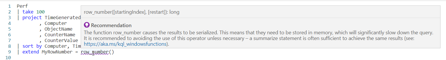
First though, if you’ve not read the introductory post on Windowing Functions, Fun With KQL Windowing Functions – Serialize and Row_Number, you should do so now as it introduced several important concepts needed to understand how these Windowing Functions work.

The samples in this post will be run inside the LogAnalytics demo site found at https://aka.ms/LADemo. This demo site has been provided by Microsoft and can be used to learn the Kusto Query Language at no cost to you.

If you’ve not read my introductory post in this KQL series, I’d advise you to do so now. It describes the user interface in detail. You’ll find it at https://arcanecode.com/2022/04/11/fun-with-kql-the-kusto-query-language/.

Note that my output may not look exactly like yours when you run the sample queries for several reasons. First, Microsoft only keeps a few days of demo data, which are constantly updated, so the dates and sample data won’t match the screen shots.

Second, I’ll be using the column tool (discussed in the introductory post) to limit the output to just the columns needed to demonstrate the query. Finally, Microsoft may make changes to both the user interface and the data structures between the time I write this and when you read it.

Row_CumSum Basics

For this example I’ll be using let to generate a simple dataset using the datatable operator. It will have two columns, the row number rowNum, and a value rowVal. For more information on let, datatable, serialize, and other functions used in this post refer to the See Also later in this post.

Using row_cumsum is simple. First, we need to pipe the dataset SomeData into a serialize so we can use it with Windowing Functions. The serialize also lets us create a new column we named cumSum, and set it equal to the row_cumsum output. As a parameter, I pass in the numeric column I want to add up, here I used the rowNum column.

As you can see in row 1, the row number (rowNum) has a value of 1. There is no data since there are no previous rows, so it just returns 1.

In the second row, the value of rowNum is 2. The cumSum column already had a value of 1, so we’ll add 2 to it, for a result of 3.

With the third row, we’ll add the value in rowNum (3) to the value in cumSum (which also happened to be 3) and we’ll now have a cumulative sum of 6.

This repeats for each row, creating a cumulative summary.

You can also create a way to decrement the data by using a negative value for the row_cumsum parameter. For example, row_cumsum(rowNum * -1) could have been used to create a decrementing value much as spending money out of your checking account would decrement your balance. You’d just want to determine the best way to handle the beginning value (first row) of the dataset.

Resetting the Cumulative Counter

It’s possible you may not want to keep accumulating for all rows, but instead only have the accumulation for a group of rows. A common task is to reset the sum when a computer name changes, or perhaps the calendar month.

For this example, I’ve added a third column to our datatable, rowBucket. Whenever the value in rowBucket changes, I want to reset the cumulative sum value.

The row_cumsum supports a second parameter that is a boolean value. When true, the counter resets. Here, I’m using an equation to calculate “is the current rows rowBucket value not equal to the one from the previous row”. If this is true, in other words not equal, then the counter will reset.

Sure enough, on row 4 the rowBucket changed to 2. On this row the cumulative sum reset itself. It now keeps adding up until the bucket number changes again, as it does with row 6.

A Real World Example

Using a datatable made the examples easy to understand, but it’s time to look at an example you might want to use in the “real world”.

Let’s imagine a scenario where you’ve detected a large amount of network traffic coming from one of the computers on your Azure network. You’d like to check the performance log table (Perf) to see how many bytes each computer sent in the last five minutes.

You need to see the number of bytes sent by a computer for each log entry, but you also want to see the total bytes sent by a computer for that time period. Let’s look at a query to accomplish this goal.

We begin with our old buddy the Perf table. A where will limit the data to the last five minutes. A second where will limit the counter to just the one we are interested in, Bytes Sent/sec. Since we only need to see this data when the virtual Azure server sent data, we’ll add a final where to remove any rows where the CounterValue is zero.

Next, we’ll use a project to strip down the columns to only the three we are interested in: the Computer, TimeGenerated, and CounterValue.

We then want to use a sort, so the data for each computer will be grouped together, then within a Computer the time the performance data was generated. Note that since the default for a sort is descending order, an asc was added after the TimeGenerated so the entries would go from the oldest to the most recent.

I normally might include an asc after the Computer so the computer names would be sorted alphabetically from A to Z, but left it off for this example just to remind you that with a sort you can mix and match the asc and desc columns.

Using a sort has another benefit. If you did go back and read my post Fun With KQL Windowing Functions – Serialize and Row_Number as I suggested in the introduction, you’ll know that the sort marks a dataset as safe for serialzation. In order to use Windowing Functions, such as row_cumsum and prev, a dataset needs to be safe for serialization.

The final line of the query is where the magic happens. Since using sort eliminated the need to use serialize, we can just use an extend to create a new column. I chose to name it cumulativeBytes.

We assign it the output of our row_cumsum Windowing Function. In the first parameter we pass in the CounterValue. In the second column we create an expression that will evaluate to true or false. We compare the Computer column for the current row and call the prev Windowing Function to get the Computer from the previous row of data.

If they are not equal, then the equation returns true. This will cause the row_cumsum to reset the cumulative sum.

Looking at the output, you can indeed see that occurred. The first computer in the list is CH1-VM-CTS. With each row it begins accumulating the CounterValue into the cumulativeBytes column.

When the Computer changed to CH-DMAVM, you can see the cumulativeBytes counter was reset. It kept accumulating the values for CH-DMAVM until the Computer changed to CH-AVSMGMTVM at which point it was again reset, and the pattern continues.

Conclusion

Cumulative sums are not an uncommon need when retrieving data. Kusto provides this ability with the Windowing Function row_cumsum, which you saw how to use in this post.

Our next post will continue the coverage of Kusto Windowing Functions by looking at the row_rank_min function.

The demos in this series of blog posts were inspired by my Pluralsight courses on the Kusto Query Language, part of their Kusto Learning Path.

There are three courses in this series so far:

I have two previous Kusto courses on Pluralsight as well. They are older courses but still valid.

These are a few of the many courses I have on Pluralsight. All of my courses are linked on my About Me page.

If you don’t have a Pluralsight subscription, just go to my list of courses on Pluralsight. On the page is a Try For Free button you can use to get a free 10 day subscription to Pluralsight, with which you can watch my courses, or any other course on the site.

Fun With KQL Windowing Functions – Prev and Next

Introduction

In this post we’ll continue our series on Kusto’s Windowing Functions by covering prev and next. If you’ve not read the introductory post, Fun With KQL Windowing Functions – Serialize and Row_Number, you should do so now as it introduced several important concepts needed to understand how these functions are used.

So what do prev and next do? They allow you to retrieve a value in a column from a previous row, or the next (or upcoming) row. This can be very useful in many situations. For instance, calculating the time between two rows based on a datetime column, or the change in a value from one row to the next.

If you’ve not read my introductory post in this series, I’d advise you to do so now. It describes the user interface in detail. You’ll find it at https://arcanecode.com/2022/04/11/fun-with-kql-the-kusto-query-language/.

Prev Basics

To make these examples simple, I’m going to use the datatable operator to generate a very simple dataset. For more on how datatable works, please see my post Fun With KQL – Datatable.

Using a let, I’ve created a dataset named SomeData. It has nine rows and two columns: rowNum and rowVal.

After my let, I take the SomeData dataset and pipe it into a serialize so it can be used with Windowing Functions like prev. Refer back to my previous post on serialize for more information on how serializing a dataset lets you use Windowing Functions.

Now the data pipes into an extend, where we add a new column I named prvVal (short for previous value). We then use strcat to combine a text string, Previous Value was with the output of our prev Windowing Function.

Into prev we pass one parameter, the name of the column from the previous row we want the data for. Here we want to pull data from the column rowVal.

As you can see in the output, the right most column displays our Previous Value was text string, plus the value from the rowVal column in the previous row.

Even More Previous

We can go back more than just one row. The prev function supports a second parameter that indicates the number of rows to go back.

First, I decided to use two extends. The first will copy the previous value into a variable, prvVal2. Into the prev function I pass two values, the first is the column name we want the data from. Here we’ll use rowVal again. The second parameter is the number of rows we want to go back, in this case we just used the value of 2.

In the next extend I user strcat to combine the prvVal2 variable with a text string and put it into the new column prvValOutput. I did this just to demonstrate you could pull a value from a previous row and use it in the query. I could have done other things with prvVal2, such as use it in a calculation.

Previous Value? What Previous Value?

You probably noticed that when we are on the first row, there is no previous value. Likewise, when on the first or second rows, and going back two there was no data. In this case the prev just returned a null value.

In the past I’ve written about functions like iif and isnull to help handle null values. Fortunately, prev eliminates the need for these as it supports and optional third parameter. Into it you can supply a value to use when the value returned by prev would otherwise be null.

In our prev we first pass the column from the previous row we want the data from, rowVal. In this example we are only going to go back one row, but since we want to use the third parameter we have to supply a value in the second parameter position. In this example we’ll use the number 1.

Finally in our third parameter we supply a value to be returned when the result of a prev would be null. Here we used the text not valid for this row, although we could have used a different datatype such as a numeric value or a datetime if that would have been more appropriate to our query.

Next, let’s look at next. The next function behaves just like prev, except it will get data from the next row in our serialized dataset instead of a previous row.

Just like with prev, as the parameter to next we pass in the name of the column to get the data from.

The next function also supports the optional second and third parameters. The second being a number indicating how many rows to go forward, the third being a value to use when next would otherwise return a null value.

Since you’ve already seen these in play I won’t create samples here, but you should be able to easily create them for yourself following the examples from prev.

Calculating a Moving Average

So it’s time for a more realistic example. Here I want to get the % Processor Time from the Perf table for a particular computer. I’m going to summarize it by hour. Then I want to create a moving average for the last three hours.

Most of the query will be pretty straightforward if you’ve been following my KQL series. I capture a start and end time using let. I then use the Perf table, followed by several where statements to limit the data.

Next I use summarize to create an average, bucketed by hour. In essence I’ll have an average of all the processor times for the 1 am hour, then 2 am, and so on.

After that we’ll sort them by the time of the day. Not only will the sort put the data in the order we want, it will also mark them as serialized. This means we can use them with our Window Function prev.

The last line is where the exciting things happen, so take a look and we’ll break it down.

We begin with extend in order to create a new column, movAvg. We are then going to add three values. The first value is the PctCpuTime from the current row, which was calculated during the summarize.

Next, I want to add in the PctCpuTime from the previous row. To do that we’ll use the prev function, pass in the PctCpuTime as the column to get, 1 to indicate we want to go back one row, then tell it to return a 0 (zero) when the previous row would return null.

This is then repeated only we pass in a value of 2, indicating we should go back two rows.

After the closing parentheses we divide by 3.0. Note its important to include the .0 otherwise it would try to create an integer output and we want a full decimal value.

And there you go, we now have an average for the last three rows of data.

Let me acknowledge, by returning a 0 for missing (null) values from the prev, the averages for the first two rows will be off. In a real world situation you’d want to make sure to take this into account, creating a solution appropriate to your situation. For this example I used zero in order to keep things simple.

Conclusion

This post continued our journey with KQL Windowing Functions, seeing how the useful prev and next functions could get data from adjacent rows of a serialized dataset. In our next post we’ll be looking at a Windowing Function to let us get cumulative sums.

The demos in this series of blog posts were inspired by my Pluralsight courses on the Kusto Query Language, part of their Kusto Learning Path.

There are three courses in this series so far:

I have two previous Kusto courses on Pluralsight as well. They are older courses but still valid.

These are a few of the many courses I have on Pluralsight. All of my courses are linked on my About Me page.

Fun With KQL Windowing Functions – Serialize and Row_Number

Introduction

The Kusto Query Language includes a set of functions collectively known as Window Functions. These special functions allow you to take a row and put it in context of the entire dataset. For example, creating row numbers, getting a value from the previous row, or maybe the next row.

In order for Window Functions to work, the dataset must be serialized. In this post we’ll cover what serialization is and how to create serialized datasets. This is a foundational post, as we’ll be referring back to it in future posts that will cover some of the KQL Windowing Functions.

Serialization

When a dataset is serialized, its data is placed in a specific order and that order is retained as the dataset goes through various transformations. Some of the Windowing Functions that require a serialized dataset to work are row_number, next, and prev to name just a few that will be covered in this and future posts.

There are some KQL functions that by their nature emit a dataset that is already ordered, in other words serialized. These include functions that I’ve already written about such as top and sort.

There are also some operators that if they receive a serialized dataset as input, will preserve the serialized ordering when the data is output. I’ve written about all of these in past posts, and they include: extend, mv-expand, parse, project, project-away, project-rename, take and where.

So the big question is, what if I need to use a Window Function but my data is not already serialized?

The Serialize Operator

For situations when you do not have an already serialized dataset you can easily create one using the serialize operator. Here’s a simple example.

All we have to do is take our dataset and pipe it into the serialize operator. The dataset will then have its order preserved, and will mark the dataset safe for use with KQLs Windowing Functions, similar to when a social media site lets you mark yourself safe from a hurricane, tornado, or all night HeavyDSparks marathon on YouTube. (#GuiltyPleasures)

Of course we don’t see any visible change here, but now we can use it with a Windowing Function. If you peeked at the post title, you’ve probably guessed already that for this post we’ll use the Window Function row_number.

But first…

A Warning!

Eagle eyed readers may notice the serialze in the screen shot above is underlined with red squiggles. This indicates there is a warning associated with this operator.

If we hover over the serialize operator the interface will display the specific warning to us.

It’s letting us know that in addition to being marked safe for Kusto Window Functions, the dataset will also be stored in memory. This could adversely affect the query runtime.

Sometimes it’s necessary to use serialize in order to get the results you need, but keep it in mind. Should you have a slow running query think about reducing the size of the dataset or see if there are other ways to accomplish the same results.

That said, let’s see how to use a basic Window Function, the row_number.

Row_Number

Calling the row_number function is easy. After the serialize operator we first provide a new column name that will hold our row number, here I used MyRowNumber. I then assign it the function row_number(). Note because it is a function we have to include the parenthesis after the function name.

In the very right most column you can see our new row number column, MyRowNumber. The value is incremented with each row.

Row_Number Without Serialize

It’s possible to call the row_number function without using the serialize operator. As discussed earlier in this post the Windowing Functions need a serialized dataset to work with, and there are a few operators that will produce a dataset that is already safe to be serialized, such as top and sort.

In addition we have the operators that will preserve serialization when a serialized dataset is passed in. As a refresher these operators include: extend, mv-expand, parse, project, project-away, project-rename, take and where.

In this example, we’ll use a sort to get our data in the order we want, then use an extend to add the new MyRowNumber column by calling the row_number() function.

As you can see, after the sort we call extend and use the same syntax as before, creating the new column of MyRowNumber and assigning it the function row_number(). Looking to the right you can see the new MyRowNumber column in the output.

You also may notice the row_number function now has a red squiggly line under it, indicating a warming. Let’s go see what that’s all about…

Another Warning!

Hovering over the row_number displays the following warning:

This warning is similar to the one you saw when we used the serialzie operator. It states that by calling row_number the data will be stored in memory, which could slow down the query.

It does have an interesting implication though. Using sort means the data can be serialized, but doesn’t mean it is. The warning states it’s the calling of a Windowing Function, such as our new friend row_number, that actually triggers the data to be serialized.

Serialize and Window Functions Recap

When we talk about Windowing Functions, I wanted to stress an important point. The serialize operator is used to convert a dataset that is not already safe for serialization into one that is. The serialization is required in order to use a Windowing Function such as row_number or one of the other’s we’ll cover in this series.

There are a list of other operators though that output data that is already safe for serialization, in other words if we use one of these operators then we can use a Windowing Function without the need to use serialize. I mentioned top and sort already, but for completeness here is the full list.

top
sort
range
getschema
top-hitters

I’ve already done blog posts for the first two (you can click on the command to follow the link to the post), and have one planned for range. If there’s interest I may cover the other two.

For completeness, let me go ahead and list the operators that will preserve the serialized state of the data when used. Note each is linked to a blog post I’ve done previously which covers each operator.

Conclusion

In this post we learned hot to use serialize to create a dataset with which we can call one of the Kusto Languages Windowing Functions. We also learned there are a handful of operators that already produce datasets safe for serialization, and can be used with Windowing Functions without the requirement to use the serialize operator.

Finally we saw the row_number Windowing Function in action. In future posts we’ll cover more of the Windowing Functions built into the Kusto Query Language.

The demos in this series of blog posts were inspired by my Pluralsight courses on the Kusto Query Language, part of their Kusto Learning Path.

There are three courses in this series so far:

I have two previous Kusto courses on Pluralsight as well. They are older courses but still valid.

These are a few of the many courses I have on Pluralsight. All of my courses are linked on my About Me page.

Fun With KQL – Datatable and Calculations

Introduction

In the conclusion of my last post, Fun With KQL – Datatable, I mentioned a datatable can also be useful when you need to do special calculations. I decided it really needed further explanation and created this post to dive in a bit deeper.

If you haven’t read my datatable post yet, you should as I’ll refer back to it. Go ahead, I’ll wait.

Datatable and Calculations

For this example we’ll revisit the Perf table. The Perf table has two main columns that we’ll use in this example, CounterName and CounterValue.

Our goal for this query is to multiply the CounterValue by some number, based on the CounterName. We could of course use a case or iif within the query, but that would result in a query that is long and hard to read and later modify if we need to.

Using a datatable will result in a query that is much more readable and maintainable. As the actual code for the query is a bit long I’ll place it below to make it easy to follow along. Note I’ll only skim over things we covered in the previous post, refer to it for more detailed explanations.

let CounterMultipliers = datatable (CounterName:string, Multiplier:int)
[
  "CounterName", 2,
  "restartTimeEpoch", 3,
  "memoryWorkingSetBytes", 4,
  "memoryRssBytes", 5,
  "memoryRequestBytes", 2,
  "memoryLimitBytes", 3,
  "memoryCapacityBytes", 4,
  "memoryAllocatableBytes", 5,
  "cpuUsageNanoCores", 2,
  "cpuRequestNanoCores", 3,
  "cpuLimitNanoCores", 4,
  "cpuCapacityNanoCores", 5,
  "cpuAllocatableNanoCores", 2,
  "Total Bytes Transmitted", 3,
  "Total Bytes Received", 4,
  "Logical Disk Bytes/sec", 5,
  "Free Megabytes", 2,
  "Disk Writes/sec", 3,
  "Disk Write Bytes/sec", 4,
  "Disk Transfers/sec", 5,
  "Disk Reads/sec", 2,
  "Disk Read Bytes/sec", 3,
  "Disk Bytes/sec", 4,
  "Bytes Sent/sec", 5,
  "Bytes Received/sec", 2,
  "Avg. Disk sec/Write", 3,
  "Avg. Disk sec/Transfer", 4,
  "Avg. Disk sec/Read", 5,
  "Available MBytes Memory", 2,
  "Available MBytes", 3,
  "% Used Space", 4,
  "% Processor Time", 5,
  "% Free Space", 6
];
let PerfData = view() {
Perf
| project CounterName
        , CounterValue
        , Computer
        , ObjectName
        , TimeGenerated
};
PerfData
| join CounterMultipliers on CounterName
| project CounterName
        , CounterValue
        , Multiplier
        , CounterExpanded = CounterValue * Multiplier
        , Computer
        , ObjectName
        , TimeGenerated

We begin with a let, where we will create a new datatable. I chose to name it CounterMultipliers, but we could have used any name we wanted.

The datatable will have two columns, the CounterName which is a string, and the Multiplier which I made an int.

I used a simple query to get the list of CounterName values:

Perf
| distinct CounterName
| sort by CounterName

I then copied the output into my query editor. I wrapped the names in quotes so they would be interpreted as strings. Next I have a comma, then the integer value to use for the multiplier.

Note I just picked a few random values to use here. In a real world situation this kind of operation, multiplying counter values, might not make much sense, but it will serve OK for this example.

After finishing the datatable definition I use a second let to create a temporary view on top of the Perf table and named the view PerfData. For more on this technique refer back to the Fun With KQL – Datatable post.

Now we take our PerfData view and join it to our datatable, CounterMultipliers. Note that I used the best practice of naming the counter name column in the datatable the same as in the PerfData view. It makes the query easier to read, and avoids the need for $left and $right as I described in the previous post.

Finally we pipe the output of the join into a project operator. I return all the columns, but add a new one, CounterExpanded. For its calculation I simply take the CounterValue column from the PerfData view and multiply it by the Multiplier column from the `datatable.

Below you can see the output from the query.

If you look in the lower right though, you will spot an issue. The query only returned 32 rows.

This demonstrates a critical piece of information when it comes to the join. For each row in the first table, PerfData, it grabs a row from the second table. Since we had 32 rows in the datatable, only 32 rows were returned.

Fixing the Query

Fixing the query is simple. All we need to do is swap the order of the two tables.

CounterMultipliers
| join PerfData on CounterName
| project CounterName
        , CounterValue
        , Multiplier
        , CounterExpanded = CounterValue * Multiplier
        , Computer
        , ObjectName
        , TimeGenerated

Note I only included the last part of the query, everything above this piece is still the same.

Now look at the output.

In the lower right, as well as in the blue area at the top of the output, you can see over 300,000 rows were returned. This is the output we expect, every row in the Perf table (from the view) linked to each row in the CounterMultipliers datatable.

Including and Excluding Columns

In this example, in the output I included the Multiplier column. This was done so you could see the data and test the calculation for yourself. In a normal situation you likely wouldn’t be doing this.

I also included the CounterValue column. Again, this may or may not be needed, you could choose to have just the CounterExpanded column.

Think about the output, and how it will be used to decide if you want to include these types of columns in your query output.

Conclusion

In this post we learned how to use a datatable to create calculated values. This made the code much cleaner, and easier to read.

The demos in this series of blog posts were inspired by my Pluralsight courses on the Kusto Query Language, part of their Kusto Learning Path.

There are three courses in this series so far:

I have two previous Kusto courses on Pluralsight as well. They are older courses but still valid.

These are a few of the many courses I have on Pluralsight. All of my courses are linked on my About Me page.

Fun With KQL – Datatable

Introduction

As you’ve seen with the join in my Fun With KQL – Join post it can be useful to combine two tables in order to clarify the output. What if, though, you need data that isn’t in an existing table?

That’s where the datatable operator comes into use. The datatable allows you to create a table of data right within the query. We’ll see a few useful examples in this post.

DataTable Basics

Let’s say you have a table that stores colors. These colors though are stored in decimal format, the application that uses them converts them to an HTML hex color. For our report though, we’d like to convert these to a friendly name, which is not stored in the source data.

To accomplish this we can create a color table with the codes as well as friendly color names. We’ll use the datatable operator to do this.

We’ll need to use our old friend let. Following we declare a name for our datatable, here we used HTMLColors although we could use any name we want.

After the equal sign we use the datatable operator. In the parenthesis we declare our column names and their data types. The first is Name, then a colon, then the data type of string. Our second column is also a string, with the name of HexCode.

The final column is DecimalValue, and its datatype is int. You can find a complete list of Kusto data types in the Microsoft documentation, Scalar data types.

After we finish the datatable declaration with a closing right parenthesis, we have an opening square bracket then declare our data. Here I put each row of data on a line by itself, this is a good practice to make it easy to read and modify.

As you can see, our first row is:

"Red",	"#FF0000", 16711680,

First is what I call our friendly name associated with the color, followed by a comma. We wrapped it in double quotes, since it is a string datatype.

Then we have the hex color code, also wrapped in quotes to make it a string, followed by a comma. Finally comes the decimal value, which is just an integer number, no quotes required.

Then line ends in a comma, then we proceed to the next line of data. At the end of our data, the row with Aquamarine, we do not have a comma since that is the last row of data. We have a closing square bracket to finish off the datatable data, then a semicolon as the KQL query will continue.

Next have the name of our datatable, piped into a project, then we listed the three columns in the datatable.

As you can see in the image above, the output section has a list of colors, hex values, and decimal value. Note that a few scrolled off the bottom of the screen.

Now we could join this to a table, linking on the DecimalValue column and display the friendly Name column in the output.

Datatable In Practice

Let’s look at an example of the datatable in practice. The Perf table has a column, ComputerName. A lot of the computer names are rather cryptic though. It’d be nice to have a friendly, human readable name that clearly says what the computer is used for, rather than unclear like JBOX10.

Let’s take a look at the query needed to add friendly names to our Perf table output.

We begin with a let and define a datatable we’ll call computers. It will have two columns, ComputerName and FriendlyName, both of which are strings.

We fall into our data, each line is simply the computer name as found in the Perf table, followed by the friendly name we want to use.

Next comes another let in which we create a datatable from Perf for the last five minutes, and use project to pick out a few columns. We’ve named this datatable PerfInfo.

Now we take our computer datatable and join it to PerfInfo. Because the column we are joining on has different names in each table, I had to use the $left and $right, as described in my Fun With KQL – Join post.

We then project the columns we want, and use sort to order the output.

I should mention I just guessed at the friendly names for some of the computer names in the Perf table. I have no idea if JBOX10 is really the XBox Java Server, but it just sounded good for this demo.

Naming DataTable Columns

I just wanted to mention that normally I would use the same column name in the datatable that is used in the table I’m joining. For example, I would use just Computer in the datatable so it would match up with the Computer column in the Perf table. That way I wouldn’t have to use the $left and $right syntax.

For this example though, I deliberately used a different name so I could remind you of the ability to use $left and $right to join tables when the column name is different.

The most frequent time you’d need this is when you are joining multiple tables with different column names for the same data, which as anyone who has worked with databases for any length of time happens far too often.

Again, for more information on this technique see my Fun With KQL – Join post.

Conclusion

The datatable can be a useful operator for situations where you want to provide user friendly names, but don’t have an existing table that contains them.

It could also be used if you needed to do calculations. For example, rather than using iif statements you could create a datatable with a country code and a standard shipping amount, then in the table use that shipping amount in a calculation, perhaps adding it to the total value of a purchase.

The demos in this series of blog posts were inspired by my Pluralsight courses Kusto Query Language (KQL) from Scratch and Introduction to the Azure Data Migration Service, two of the many courses I have on Pluralsight. All of my courses are linked on my About Me page.

If you don’t have a Pluralsight subscription, just go to my list of courses on Pluralsight . At the top is a Try For Free button you can use to get a free 10 day subscription to Pluralsight, with which you can watch my courses, or any other course on the site.