Introduction
I’m still working on my ArcaneBooks project, mostly documentation, so I thought I’d take a quick break and go back to a few posts on KQL (Kusto Query Language). In this post we’ll cover the join operator.
A join in KQL operates much as it does in SQL. It will join two datasets together into a single result.
The samples in this post will be run inside the LogAnalytics demo site found at https://aka.ms/LADemo. This demo site has been provided by Microsoft and can be used to learn the Kusto Query Language at no cost to you.
If you’ve not read my introductory post in this series, I’d advise you to do so now. It describes the user interface in detail. You’ll find it at https://arcanecode.com/2022/04/11/fun-with-kql-the-kusto-query-language/.
Note that my output may not look exactly like yours when you run the sample queries for several reasons. First, Microsoft only keeps a few days of demo data, which are constantly updated, so the dates and sample data won’t match the screen shots.
Second, I’ll be using the column tool (discussed in the introductory post) to limit the output to just the columns needed to demonstrate the query. Finally, Microsoft may make changes to both the user interface and the data structures between the time I write this and when you read it.
A Basic Join
Here is a basic join. Since the image is a bit small I’ll reproduce the query first.
Perf
| where TimeGenerated >= ago(30d)
| take 1000
| join (Alert) on Computer
We start with the first table, Perf. We use a where to limit the data to the last thirty days, then use take to grab 1000 rows.
Then comes the join. After the join comes the table we want to join to, enclosed in parethesis. In this case we are joining to the Alert table.
After the table name we have the keyword on, then the column name to use for the join, here Computer.
Here you can see the query returned three rows. The first set of columns come from the Perf table. There is a second TimeGenerated (UTC) column, this came from the Alert table, as well as the rows to the right of it. Note there are more columns that are off to the right.
A More Complex Join
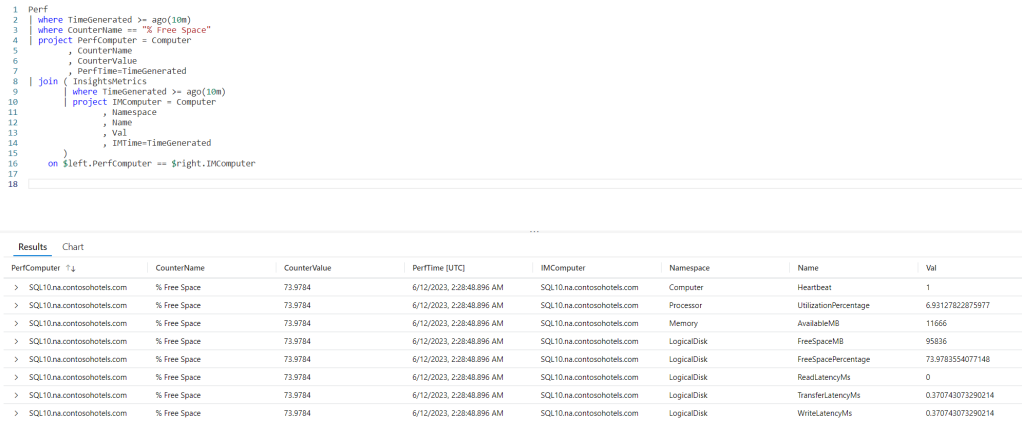
Here we have a more complex, and realistic join. Because the image is a bit small I’ll reproduce it below.
Perf
| where TimeGenerated >= ago(10m)
| where CounterName == "% Free Space"
| project PerfComputer = Computer
        , CounterName
        , CounterValue
        , PerfTime=TimeGenerated
| join ( InsightsMetrics
       | where TimeGenerated >= ago(10m)
       | project IMComputer = Computer
               , Namespace
               , Name
               , Val
               , IMTime=TimeGenerated
       )
    on $left.PerfComputer == $right.IMComputer
We grab the Perf table, and use some where statements to limit the results. The query then falls into a project so we can limit the number of columns. Note we are renaming two of the columns, the Computer and TimeGenerated.
Next comes the join. In parenthesis we have a second query that access the InsightsMetrics table. We have a where, then a project. Within it we rename the Computer and TimeGenerated columns.
Next we have the on, followed by the columns to join on. Because we are joining on different column names we need to specify both names, and use == to show they match.
We also have to indicate which sides of the query the columns come from. To do so we prefix the column names with $left and $right. The left side is the first query coming into the join, the right side will be the second query.
Here is the query, with the results.
Note that in a real world query we’d probably want to add the TimeGenerated to the query, and perhaps other columns, but I kept it to just one for simplicity. If we had more, we would just add the conditions after a comma.
Join Types
Similar to SQL, join supports multiple types. By default it uses an innerunique, but there are quite a few.
- fullouter
- inner
- innerunique
- leftanti
- leftantisemi
- leftouter
- leftsemi
- rightanti
- rightantisemi
- rightouter
- rightsemi
To use one of these, after the join just specify the kind.
join kind=fullouter
Join Kind Reference
Below is an explanation of the various types of joins.
- innerunique
Only one row from the left is matched for each value of the on key. Output contains a match for each row on the right with a row on the left. NOTE: This is the default. If you are coming from a SQL background, you might expect the behavior to be inner, so be careful to look over your results. If you wanted a SQL style inner join you will need to
explicitly specify kind=inner when you execute the query!
- inner
Output has one row for every combination of left and right.
- leftouter
In addition to every match, there’s a row for every row on the left even if there’s no match on the right
- rightouter / fullouter
Same as left outer, but either includes all rows from the right side, or all rows, regardless of matches.
- leftanti / rightanti
The reverse of outer joins, only returns rows who do NOT have a match on the right (or left depending on which was used).
- leftsemi / rightsemi
Returns rows who have a match on both sides, but only includes the columns from the left side (or right if rightsemi was used)
A Complex Example
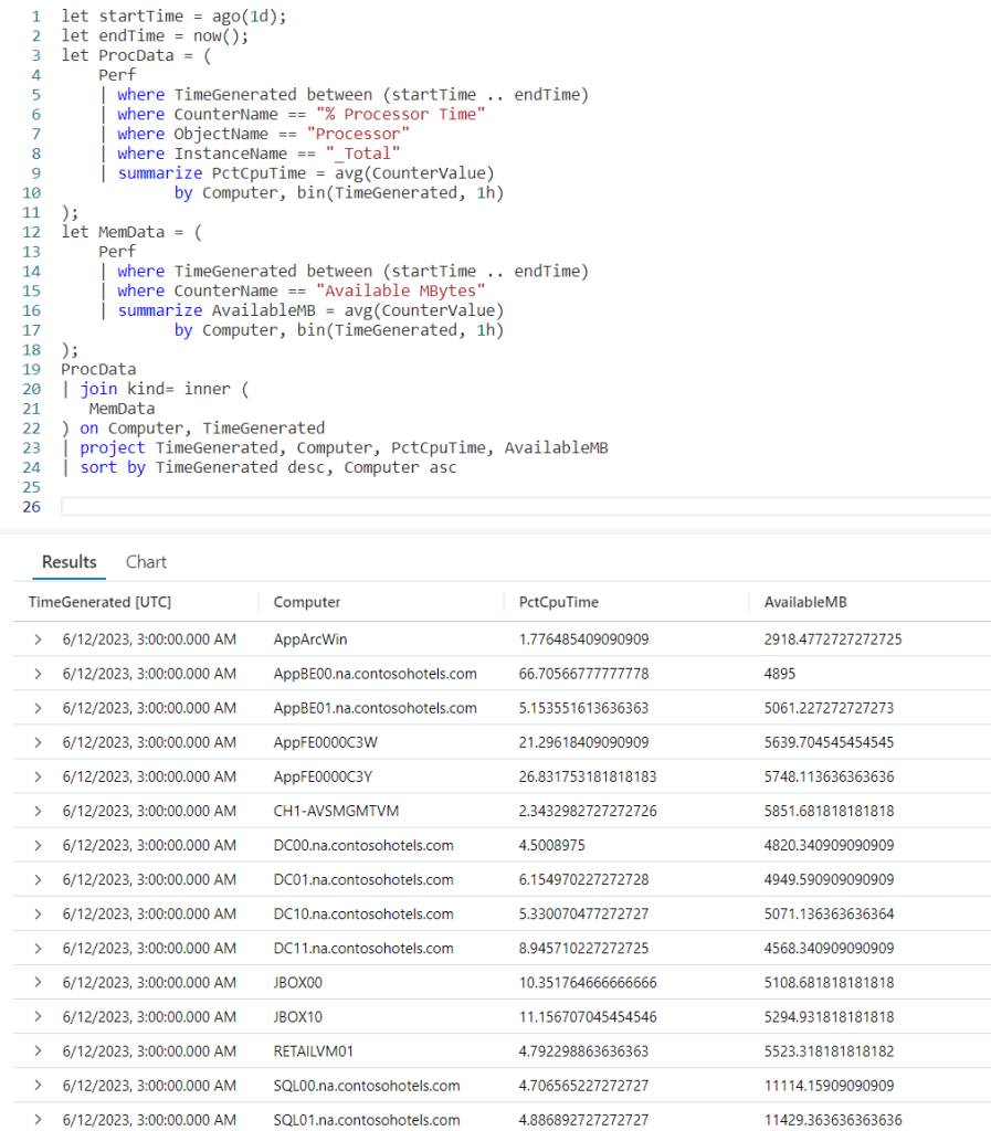
Let’s wrap this up with a more complex example. This query will make use of the let operator which I covered in my pervious post on KQL.
We start with two let statements to set the start and end time ranges. This will make it easy to update these when we need to use the query in the future. Note that we need to end each line in a semicolon since we have multiple KQL queries we are joining together to make our ultimate query.
The next let will create a new datatable and store the result of a query. We give it a name, ProcData, then assign it by creating a valid KQL query within parenthesis.
We repeat to create a second datatable, named MemData. Again note the use of semicolons.
Now we fall into the main query. By using the datatable names it makes the join query very easy to read. After the main query we fall into a project to limit the output columns, then a sort to get the columns in the order we want.
let startTime = ago(1d);
let endTime = now();
let ProcData = (
    Perf
    | where TimeGenerated between (startTime .. endTime)
    | where CounterName == "% Processor Time"
    | where ObjectName == "Processor"
    | where InstanceName == "_Total"
    | summarize PctCpuTime = avg(CounterValue)
            by Computer, bin(TimeGenerated, 1h)
);
let MemData = (
    Perf
    | where TimeGenerated between (startTime .. endTime)
    | where CounterName == "Available MBytes"
    | summarize AvailableMB = avg(CounterValue)
            by Computer, bin(TimeGenerated, 1h)
);
ProcData
| join kind= inner (
   MemData
) on Computer, TimeGenerated
| project TimeGenerated, Computer, PctCpuTime, AvailableMB
| sort by TimeGenerated desc, Computer asc
Here is the result of the query.
See Also
The following operators, functions, and/or plugins were used or mentioned in this article’s demos. You can learn more about them in some of my previous posts, linked below.
Conclusion
In this post, we learned how to use a join operator to merge two tables together.
The demos in this series of blog posts were inspired by my Pluralsight courses Kusto Query Language (KQL) from Scratch and Introduction the Azure Data Migration Service, two of the many courses I have on Pluralsight. All of my courses are linked on my About Me page.
If you don’t have a Pluralsight subscription, just go to my list of courses on Pluralsight . At the top is a Try For Free button you can use to get a free 10 day subscription to Pluralsight, with which you can watch my courses, or any other course on the site.


